10.3 Z-scores and p-values
Recall the Overview of Hypothesis Testing. Now, we are going to add details to help us make a final decision about the null hypothesis.
- Carry out a test of the hypothesis, such as a difference-in-means.
- Applicants with a criminal record receive 12.5 percentage points fewer call backs than those without a criminal record
- Calculate the uncertainty around this estimate.
- We will estimate the standard error of the estimate using the sample size and sample spread (standard deviation)
- We can also estimate the confidence intervals
- Decide whether you can reject or fail to reject the hypothesis of no difference
- Standarize the estimate and find the z-score (or t-statistic, which is similar)
- The z score is an example of a “test statistic.” The type of statistic might vary across applications, but its purpose will remain similar. Others include t-statistics and Chi-squared statistics.
- How likely is it you would observe the z-score you found under this null distribution? (p-value)
- If the p-value is small (\(< 0.05\)), reject the null.
- Standarize the estimate and find the z-score (or t-statistic, which is similar)
A z-score helps us standardize the size of estimates across any units of study by quantifying the size of the estimate in terms of standard errors.
z-score = \(\frac{\text{Estimate - Null}}{\hat{SE}} = \frac{\text{Estimate - 0}}{\hat{SE}}\)
The z-score represents a ratio of the estimate over the standard errors. We can visualize the distribution of z-scores in the image below.
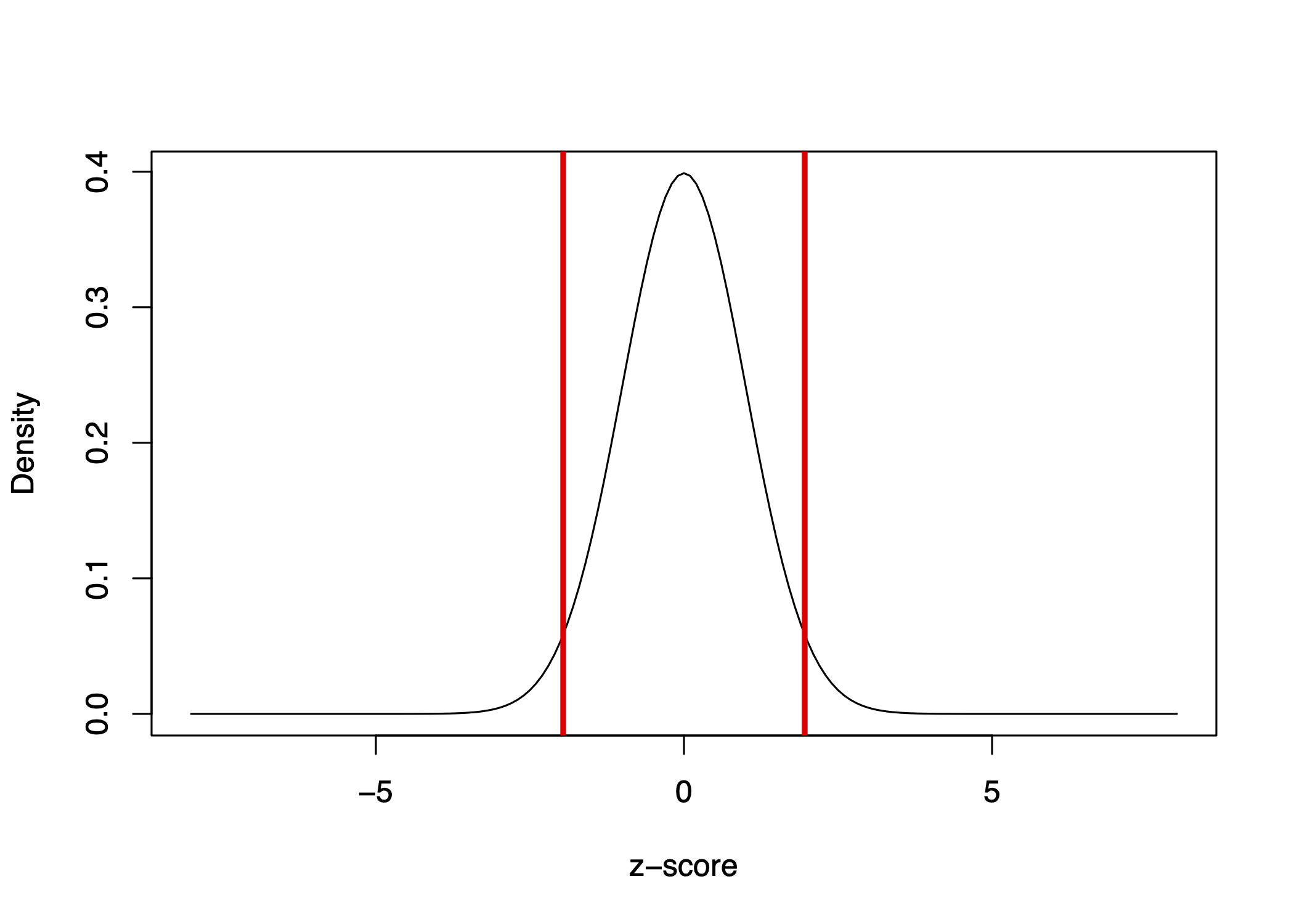
The bell curve is centered on 0 and represents our null distribution.
- Instead of the axis being the number of heads out of 100 coin flips, centered on the null hypothesis of 50 heads for a fair coin, the standardized scale is centered on 0. We can then visualize how far 80 coin flips is away from 50 in terms of standard errors.
Recall, we asked: When we conduct an experiment and find that applicants with a criminal record were called back 12.5 percentage points less often than those without a criminal record, we want to know…
- Is that a real difference, or is the real difference 0, and we just happened to get our 12.5-point difference in our sample due to random chance?
It so happens that our 12.5 percentage difference represents more than z=7.
We can visualize where z=7 is in our distribution below with the dashed purple line:
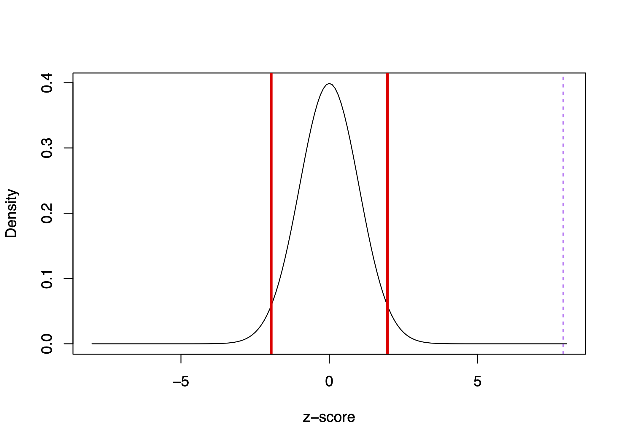
It is well outside of the red lines representing 1.96 standard errors.
Interpretation: It is really unlikely we would have observed this extreme in magnitude of difference if the true difference were 0.
- This likelihood represents the p-value, which is essentially 0 in this case. There is essentially 0 chance we would have observed a difference as large or larger than 12.5 (or -12.5) in a world where the true difference is 0.
- If a p-value is < 0.05, we reject the null hypothesis.
- If instead, the p-value is larger than 0.05, we fail to reject the null. That would mean that we think it is reasonably possible to have observed a difference as big as 12.5 if in fact the true difference is 0.
We are going to focus on two-sided p-values, which focus on the magnitude of the z-score in either direction, instead of whether it is a positive or negative p-value. In other classes, you may also cover one-sided p-values.
10.3.1 Relationship to Confidence Intervals
Relationship to Confidence Intervals: Our 12.5 percentage difference has a 95% confidence interval of 6.8 to 18.3
- It is constructed by taking \(12.5 - 1.96*SE\) and \(12.5 + 1.96*SE\)
- This means there is a 95% chance that this interval contains the true population difference.
It gives us another way of describing our estimate that includes our uncertainty. We recognize that over repeated samples, we are not always going to get a 12.5 point difference. In any given sample, this estimate will differ a bit over the “sampling distribution.”