2.4 Loading data into R
For this section, our motivating example will be methods to measure voter turnout in the United States.
Describing voter turnout
- What is a typical level of voter turnout?
- How has turnout changed over time?
- Is turnout higher in presidential years or in midterm years?
How can we measure turnout? Think about the validity, reliability, and cost of different approaches.
Example: Dataset on Voter Turnout in the U.S. across multiple years
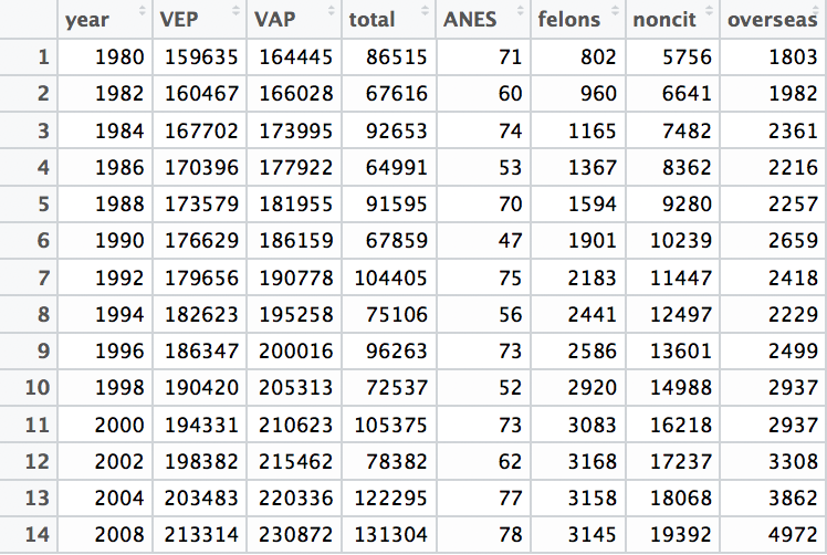
In this dataset, each row is an election year. Each column contains information about the population, potential voters, or voter turnout. These will help us compute the turnout rate in a given year. To work with this dataset, we need to load it into R.
2.4.1 Working with datasets in R
For a video explainer of the code in this section, see below. The video only discusses the code. Use the notes and lecture discussion for additional context. (Via youtube, you can speed up the playback to 1.5 or 2x speed.)
Often the variables we care about are stored inside of rectangular datasets
- These have a number of rows
nrow()and columnsncol() - Each row is an “observation,” representing the information collected from an individual or entity
- Each column is a variable, representing a changing characteristic across multiple observations
When we import a dataset into R, we have a few options.
Option 1: Download dataset to your computer
- Move the dataset to your working directory
- Identify the file type (e.g., csv, dta, RData, txt)
- Pick the appropriate R function to match the type (e.g.,
read.csv(), read.dta(), load(), read.table()) - Assign the dataset to an object. This object will now be
class()ofdata.frame
turnout <- read.csv("turnout.csv")Option 2: Read file from a url provided
- Need an active internet connection for this to work
- URL generally must be public
- Include the url inside the function used to read the data
turnout <- read.csv("https://raw.githubusercontent.com/ktmccabe/teachingdata/main/turnout.csv")class(turnout)## [1] "data.frame"You can also open up a window to view the data:
View(turnout)2.4.2 Measuring the Turnout in the US Elections
Relevant questions with voter turnout
- What is a typical level of voter turnout?
- Is turnout higher in presidential years or in midterm years?
- Is turnout higher or lower based on voting-eligible (VEP) or voting-age (VAP) populations? We have a lot of people who are citizens 18 and older who are ineligible to vote. This makes the VEP denominator smaller than the VAP.
Voter Turnout in the U.S.
- Numerator:
total: Total votes cast (in thousands) - Denominator:
- VAP: (voting-age population) from Census
- VEP (voting-eligible population) VEP = VAP + overseas voters - ineligible voters
- Additional Variables and Descriptions
year: election yearANES: ANES self-reported estimated turnout rateVEP: Voting Eligible Population (in thousands)VAP: Voting Age Population (in thousands)total: total ballots cast for highest office (in thousands)felons: total ineligible felons (in thousands)noncitizens: total non-citizens (in thousands)overseas: total eligible overseas voters (in thousands)osvoters: total ballots counted by overseas voters (in thousands)
2.4.3 Getting to know your data
## How many observations (the rows)?
nrow(turnout)
## [1] 14## How many variables (the columns)?
ncol(turnout)## [1] 9## What are the variable names?
names(turnout)## [1] "year" "VEP" "VAP" "total" "ANES" "felons" "noncit"
## [8] "overseas" "osvoters"## Show the first six rows
head(turnout)## year VEP VAP total ANES felons noncit overseas osvoters
## 1 1980 159635 164445 86515 71 802 5756 1803 NA
## 2 1982 160467 166028 67616 60 960 6641 1982 NA
## 3 1984 167702 173995 92653 74 1165 7482 2361 NA
## 4 1986 170396 177922 64991 53 1367 8362 2216 NA
## 5 1988 173579 181955 91595 70 1594 9280 2257 NA
## 6 1990 176629 186159 67859 47 1901 10239 2659 NAExtract a particular column (vector) from the data using the $.
turnout$year## [1] 1980 1982 1984 1986 1988 1990 1992 1994 1996 1998 2000 2002 2004 2008Extract the 10th year. Just like before! We use 10 to indicate the value of the year column in position (row 10) of the data.
turnout$year[10]## [1] 1998We can take the mean() of a particular column, too. Let’s take it of the total number of voters.
mean(turnout$total)## [1] 89778.29And get the class() (Note: integer is just a type of numeric variable)
class(turnout$total)## [1] "integer"We can also use brackets in the full data frame, but because our data frame has BOTH rows and columns, we cannot just supply one position i. Instead, we have to tell R which row AND which column by using a comma between the positions.
turnout[1,2] # value in row 1, column 2## [1] 159635We can use the column name instead
turnout[1, "VEP"]## [1] 159635If we leave the second entry blank, it will return all columns for the specified row
turnout[1,] # All variable values for row 1## year VEP VAP total ANES felons noncit overseas osvoters
## 1 1980 159635 164445 86515 71 802 5756 1803 NAThe opposite is true if we leave the first entry blank.
turnout[,2] # VEP for all rows## [1] 159635 160467 167702 170396 173579 176629 179656 182623 186347 190420
## [11] 194331 198382 203483 213314