8.4 Step 2: Checking accuracy of model
Understanding prediction error: Where do \(\hat \alpha\) and \(\hat \beta\) come from? Recall that a regression tries to draw a “best fit line” between the points of data.
Under the hood of the regression function, we are searching for the values of \(\hat \alpha\) and \(\hat \beta\) that try to minimize the distance between the individual points and the regression line.
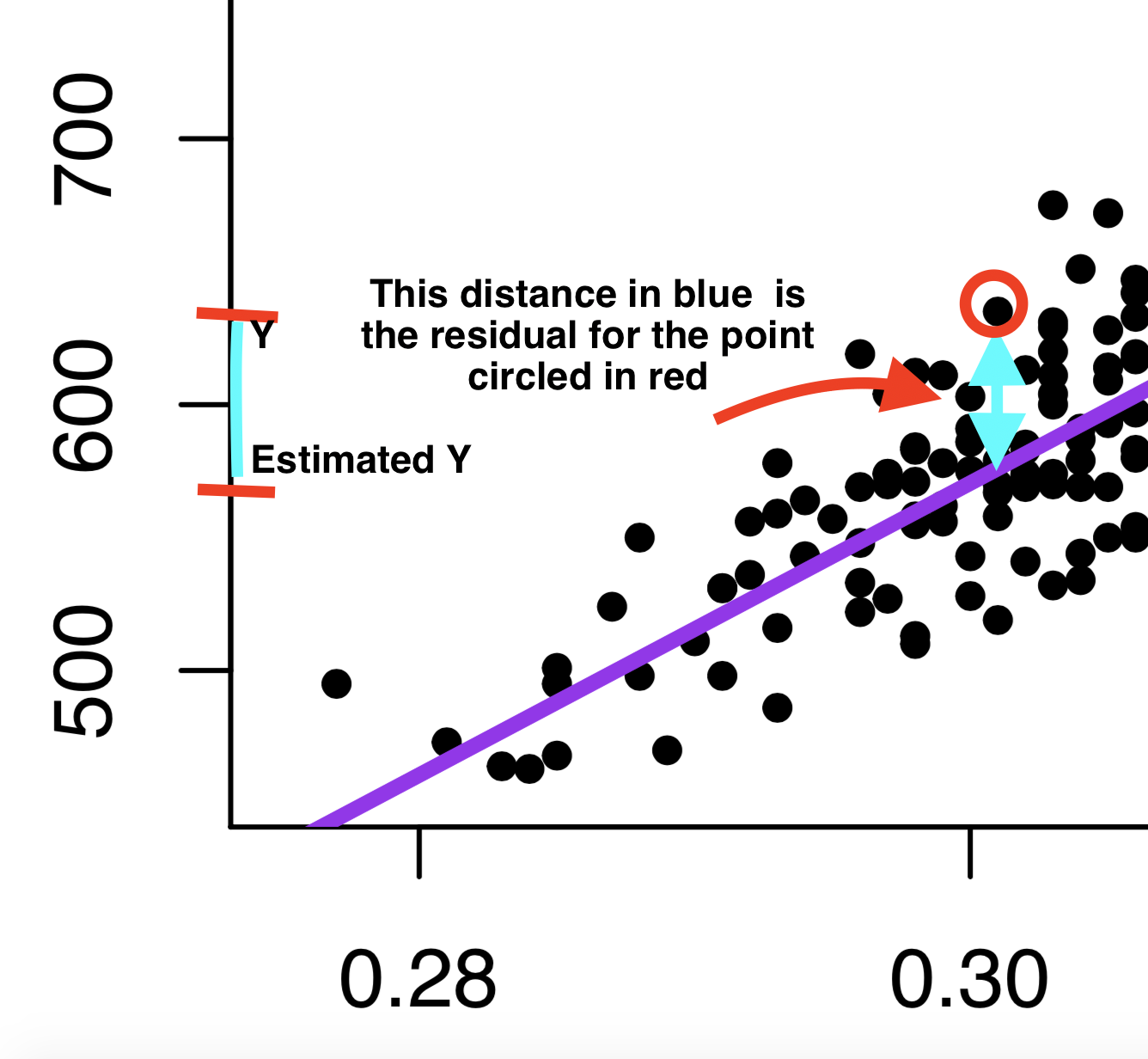
This distance is called the residual: \(\hat \epsilon_i = Y_i - \hat Y_i\).
- This is our prediction error: How far off our estimate of Y is (\(\hat Y_i\)) from the true value of Y (\(Y_i\))
- Linear regressions choose \(\hat \alpha\) and \(\hat \beta\) to minimize the “squared distance” of this error (think of this as the magnitude of the distance). This is why we tend to call this type of linear regression ordinary least squares (OLS regression).
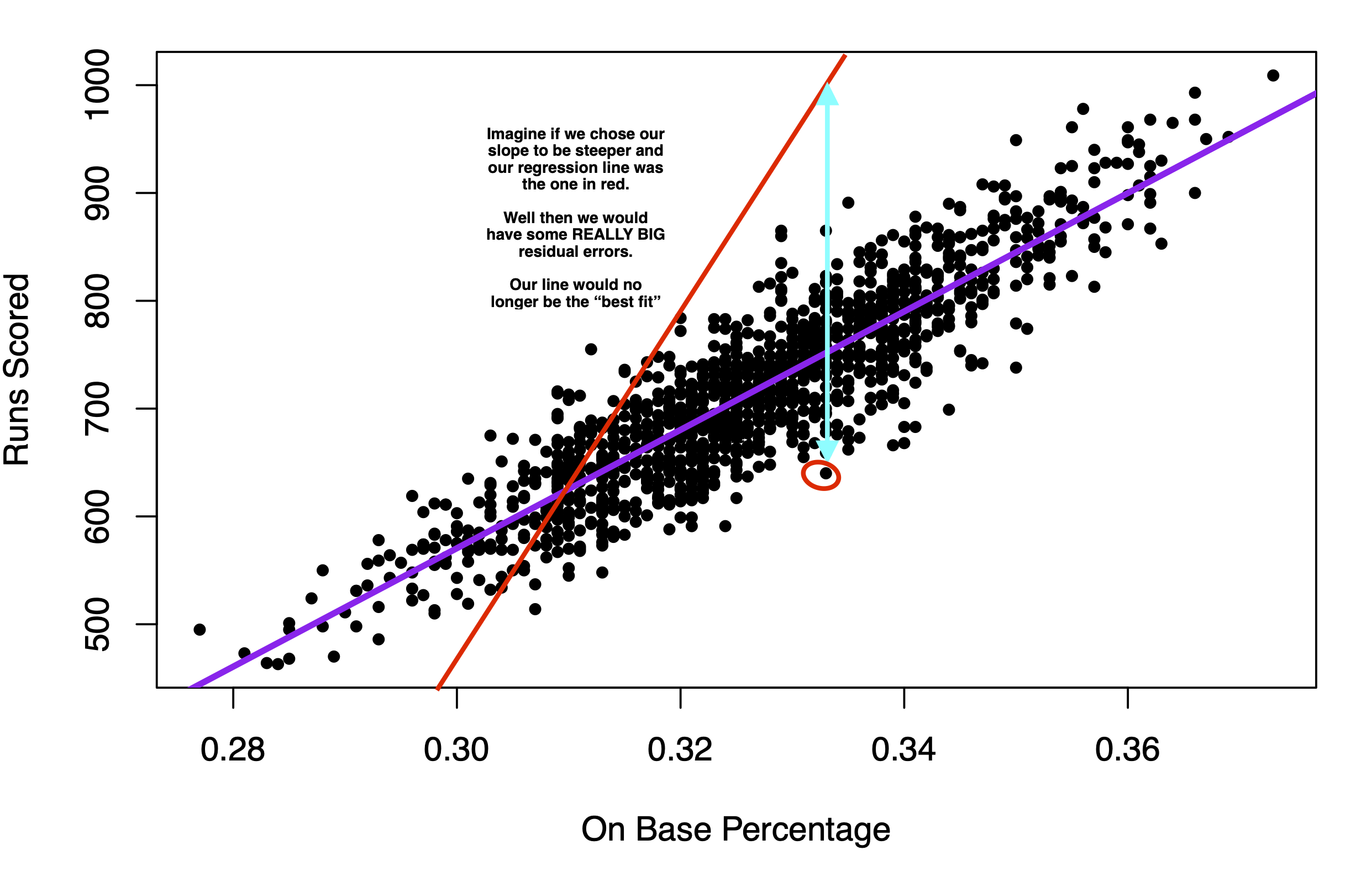
If instead we chose the red line in the image below to be the regression line, you can see that the typical prediction error would be much larger. That’s why we end up with the purple line.
8.4.1 Root Mean Squared Error
Just like we had root mean squared error in our poll predictions, we can calculate this for our regression.
- Just like with the polls, this is the square root of the mean of our squared prediction errors, or “residuals” in the case of regression
- R will give us this output automatically for a regression using
sigma()
- R will give us this output automatically for a regression using
sigma(fit)## [1] 39.82189- In our case, using on based percentage to predict runs scored, our estimates are off typically, by about 40 runs scored.
- On the graph, this means that the typical distance between a black point and the purple line is about 40.