10.2 Sampling and Uncertainty
Flip a coin 10 times here. Report how many times it lands on heads.
- Imagine repeating this process over and over again.
- We know that a fair coin should land on heads 50% of the time- 5 out of 10 times or 50 out of 100 times.
- However, in any given sample of coin flips, you might get a slightly different result. If you repeated the sample a bunch of times, sometimes you might get 4 heads, 5 heads, 6 heads, 3 heads, etc.
This does not mean the coin is unfair. Instead, just due to chance, we ended up with 6 out of 10 heads in a world where the true proportion of times that coin would land on heads is .5.
How much evidence would we need to reject the idea that the coin is unfair? What if we got 90 heads out of 100 coin flips? Would that be enough to make us skeptical of the coin?
- This is the idea of null hypothesis testing. We gather evidence and make a judgment about whether we can reject a null hypothesis. How likely would it be that by chance we could flip 90 heads in a world where that coin was actually fair?
- For example, when we find a relationship between two variables (e.g., a correlation, a difference-in-means, a regression coefficient), this could be due to chance in a single sample.
When we conduct an experiment and find that applicants with a criminal record were called back 12.5 percentage points less often than those without a criminal record, we want to know…
- Is that a real difference, or is the real difference 0, and we just happened to get our 12.5-point difference in our sample due to chance?
In statistical hypothesis testing, what we will try to do is quantify how likely it is that we could observe a difference as big as 12.5 in a given sample if, in fact, the real difference is 0. We want to be able to make a judgment about how likely the relationship we observed in a sample of applications/hiring decisions could exist in a world where criminal records really have no impact on job prospects.
We are going to use this example help us break down a few concepts.
10.2.1 Sampling Distribution
The number of heads you generate over repeated samples is the “sampling distribution.”

The higher the curve, the more likely we would observe that number of heads. For example, if you flip a coin 100 times, it is likely you will get close to 50 heads (50%), and very unlikely you will flip more than 80 heads (80% heads).
- So if you flip a coin and get 55 heads, we might still think the coin is fair, but once you start moving to the tails of this curve . . .
- It is highly unlikely we could flip a coin 100 times and get 80 heads just by random chance i.e., if the coin were fair.
- The “bell” shape of this distribution isn’t an anomaly. The “Central Limit Theorem” tells us that over repeated samples (so long as your sample is sufficiently large), the distribution of “means” will be normal
- This is incredibly important because we know a lot about normal distributions, such as that 95% of the sample mean estimates fall within two (technically: 1.96) standard errors of the mean.
- Only if we observe a number of heads outside those lines would we think perhaps it is not a fair coin.
Let’s now imagine our study on criminal records and job prospects. In a world where the true difference in call back rates between those with and without criminal records is 0, in any given sample, we might end up with a 3 percentage point difference, -5 percentage point difference, 2 point difference, -1 point difference, and so on.
- The shape of the bell curve would be centered on 0 difference (Central Limit Theorem), meaning on average, over repeated samples of applicants/hiring decisions, there would be 0 difference, but occasionally we would still find some differences across samples.
- What we want to know is if a 12.5 point difference is within two standard errors of 0 or if it is pretty unusual. (Is it more like 55 heads or 80 heads?)
10.2.1.1 Details: Standard Errors
A standard error is the standard deviation of the sampling distribution
- Where a standard deviation is the typical distance between a given observation and the mean.
- Compare the two photos below showing 0 standard deviation vs. a large standard deviation
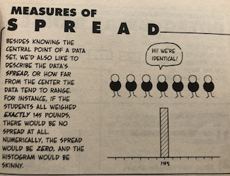
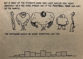
From the Cartoon Guide to Statistics
In real life studies, we don’t know the actual sampling distribution because we only have 1 sample (we only had one study of applications/hiring decisions).
So we estimate our standard error using the standard deviation of our sample (\(S\)) and sample size (\(N\)).
\({\hat {SE}} = \frac{S}{\sqrt{N}}\)
The bigger the sample, the SMALLER the standard error (which is good) because it means less uncertainty.