12.7 Week 12 Exercise
Please load donation.dta. This is a data set that includes an original survey of 2815 past campaign donors in the United States.
library(foreign)
don <- read.dta("https://github.com/ktmccabe/teachingdata/blob/main/donation.dta?raw=true")
The researchers randomly sampled survey respondents based on a list from the FEC, which contained the names of anyone who gave $200 or more to a candidate in the two years prior to 2012. The sampling process was designed to focus on donation behavior to the 22 senators who sought reelection in 2013–selecting people who might donate or might be pursued for a donation by one of these senators. The idea was that this sample would represent the senators’ potential “donorate”. Each observation is a senator-donor dyad: with 22 incumbent senators running for reelection and 2815 respondents, there are approximately 61,930 dyads (observations). For each observation, the data contain variables that indicate whether or not a respondent donated to the senator and how much that donation was, as well as the respondent’s total donations. Senators are required to record donations above $200, but some senators voluntarily report donations below this amount. Therefore, the data may include some donation totals between 0 and $200.
Key Variables include:
donation: 1=made donation to senator, 0=no donation madetotal_donation: Dollar amount of donation made by donor to Senator.total_donation_all: Dollar amount of all FEC recorded donations made by this donor.maxdon: Dollar amount of the donor’s largest donation.numsens: Number of unique senators a donor gave to.numdonation: Number of unique donations a donor gave.peragsen: policy agreement, percent issue agreement between donor and senatorper2agchal: percent issue agreement between donor and the senator’s challengercook: Cook competitiveness score for the senator’s race. 1 = Solid Dem or Solid Rep; 2 = Likely Dem or Likely Rep; 3 = Leans Dem or Leans Rep; 4 = Toss Upsame_state: 1=donor is from senator’s state, 0=otherwisesameparty: 1=self-identifies as being in the candidate’s party; 0 otherwisematchcommf: 1=Senator committee matches donor’s profession as reported in FEC file; 0=otherwiseNetWorth: Donor’s self-estimated net worth. 1=less than 250k, 2=250-500k; 3=500k-1m; 4=1-2.5m; 5=2.5-5m; 6=5-10m; 7=more than 10mIncomeLastYear: Donor’s household annual income in 2013. 1=less than 50k; 2=50-100k; 3=100-125k; 4=125-150k; 5=150-250k; 6=250-300k; 7=300-350k; 8=350-400k; 9=400-500k; 10=more than 500kidfold2: Donor’s self-described political ideology. 0 = moderate; 1=somewhat conservative or somewhat liberal; 2=conservative or liberal; 3=very liberal or very conservativenotwhite: Donor’s self-described ethnicity. 1=not white; 0=whitemalerespondent: Donor’s self-described gender. 1=male; 0=femaleterms: The number of terms a legislator has been in officeYearBorn: Donor’s year of birth.Edsum: Donor’s self-described educational attainment. 1=less than high school; 2=high school; 3=some college; 4=2-year college degree; 5=4-year college degree; 6=graduate degreeideologue2: 1=respondent suggested the candidate’s ideological position was “extremely important” or if the respondent attached more importance to this factor than to both whether the “candidate could affect my industry or work” and “I know the candidate personally”, 0=otherwiseIK2: 1=respondent suggested “I know the candidate personally” was “extremely important” or if the respondent attached more importance to this factor than to both whether the “candidate’s position on the issues is similar to mine” and “the candidate could affect my industry or work”, 0=otherwisedonor_id: donor respondent unique id (each respondent is in the data 22 times)- The data also include dummy variables for each senator (e.g.,
sendum1,sendum2)
Research Question: Does policy agreement motivate people to give to campaigns?
- Conduct and present an analysis that can help answer the question.
Try on your own, then expand to see the authors’ approach.
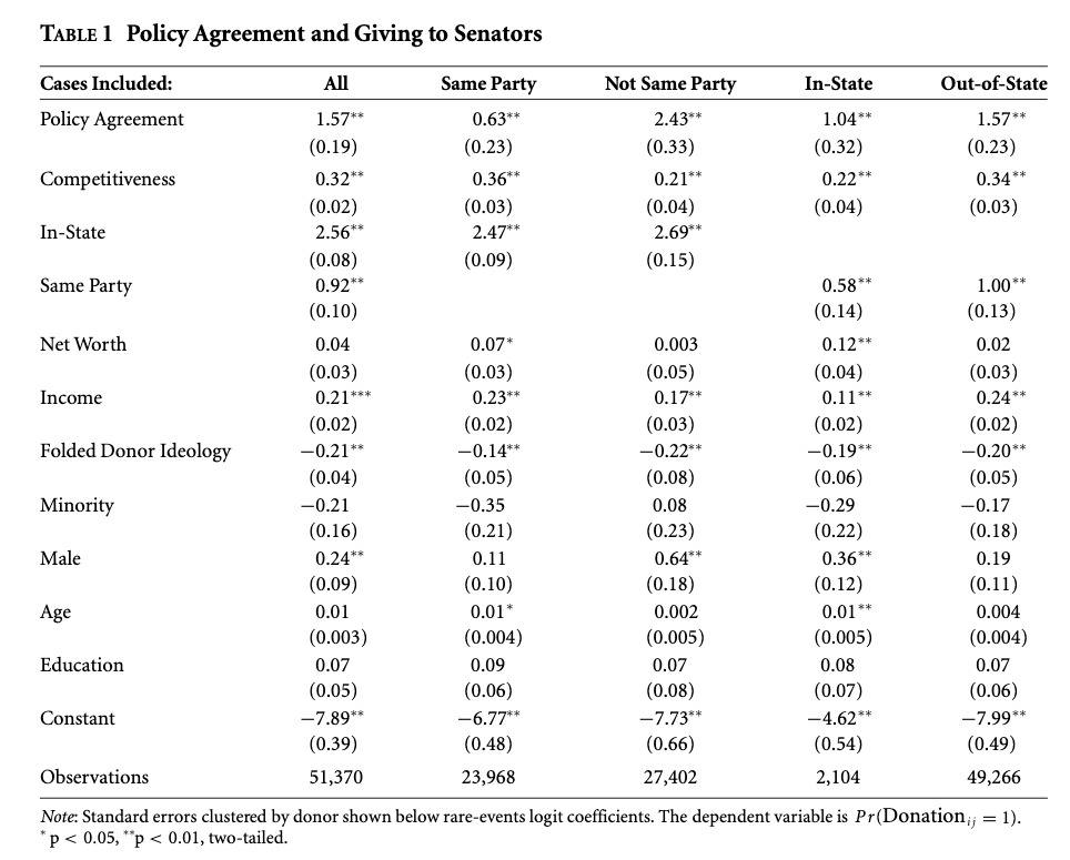
This dataset comes from “Ideologically Sophisticated Donors: WhichCandidates Do Individual Contributors Finance?” by Michael J. Barber, Brandice Canes-Wrone, and Sharece Thrower. It was published in the American Journal of Political Science in 2017.
The authors use a “rare events logit” with clustered standard errors by donor “in order to account for the fact that the decision to give to a candidate may be correlated with decisions regarding other campaigns.” They also use a standard logistic regression as a robustness check in the appendix. They conduct an analysis among the full data, as well as theoretically interesting senator-respondent combinations.
For information on rare events logits, as a special form of the logit model, see here, a response here, and R code here.
They also analyze the amount given by transforming the variable into an incremental count outcome. “Because donations tend to be given in $50 increments, we use a rank-ordered variable that equals 0 for $0, 1 for $1–$49, 2 for $50–$99, and so on. Supplemental Table A9 shows that the results are robust to using the exact dollar amount, a rank based on $100 increments, and one based on $500 increments. Because donations are capped at $5,000, all of these dependent variables reflect this maximum. Moreover, as with the probability of donating, there is an overdispersion of zeros representing cases where a donor did not give to a senator. We accordingly use a zero-inflated negative binomial regression model for analyses of the amount donated. Additionally, for purposes of comparison, we show results for Tobit specifications.”
In our live discussion, we came up with several different possibles approaches, frequently using binary logistic regression with donation as the outcome or a linear model with total_donation as the outcome. Some suggested specifications also included fixed effects for the donors using the plm package and fitting a within model. Finally, we explored using random effects in plm or lme4, though the lme4 approach appeared very stressful for our computers!
Overall, we came up with consistent support for the positive relationship between policy agreement and giving to campaigns. Here are a few approaches developed:
fit <- glm(donation ~ peragsen +
             terms + same_state +
             idfold2, data=don,
           family=binomial(link = "logit"))

fit2 <- glm(donation ~ peragsen + cook +
              NetWorth + idfold2 + notwhite + malerespondent + terms,
            data=don,
            family=binomial(link = "logit"))

fit3 <- glm(donation ~ peragsen + cook +
              NetWorth + idfold2 + notwhite + malerespondent + terms + sameparty,
            data=don,
            family=binomial(link = "logit"))

library(plm)
## remove missing data from the fixed effect to get plm to work
don2 <- subset(don, is.na(donor_id) ==F)
fit5 <- plm(total_donation ~ peragsen, data = don2,
            model = "within",
            index = c("donor_id"))

## random effects
fit6 <- plm(total_donation ~ peragsen, data = don2,
            model = "random",
index = c("donor_id"))library(texreg)
htmlreg(list(fit, fit2, fit3, fit5, fit6),
custom.model.names = c("Logit", "logit", "logit", "Lin. FE", "Lin. RE"))| Logit | logit | logit | Lin. FE | Lin. RE | |
|---|---|---|---|---|---|
| (Intercept) | -4.38*** | -6.38*** | -6.20*** | -4.40 | |
| (0.08) | (0.14) | (0.14) | (3.39) | ||
| peragsen | 2.02*** | 2.64*** | 1.62*** | 97.09*** | 90.87*** |
| (0.11) | (0.11) | (0.14) | (5.19) | (4.99) | |
| terms | -0.13*** | -0.07* | -0.05 | ||
| (0.03) | (0.03) | (0.03) | |||
| same_state | 2.65*** | ||||
| (0.05) | |||||
| idfold2 | -0.19*** | -0.17*** | -0.23*** | ||
| (0.02) | (0.02) | (0.02) | |||
| cook | 0.28*** | 0.29*** | |||
| (0.02) | (0.02) | ||||
| NetWorth | 0.22*** | 0.21*** | |||
| (0.01) | (0.01) | ||||
| notwhite | -0.37*** | -0.38*** | |||
| (0.11) | (0.11) | ||||
| malerespondent | 0.30*** | 0.32*** | |||
| (0.05) | (0.06) | ||||
| sameparty | 0.85*** | ||||
| (0.07) | |||||
| AIC | 16167.66 | 15151.83 | 14935.63 | ||
| BIC | 16212.69 | 15222.81 | 15015.45 | ||
| Log Likelihood | -8078.83 | -7567.92 | -7458.81 | ||
| Deviance | 16157.66 | 15135.83 | 14917.63 | ||
| Num. obs. | 60280 | 52734 | 52536 | 62544 | 62544 |
| R2 | 0.01 | 0.01 | |||
| Adj. R2 | -0.04 | 0.01 | |||
| s_idios | 316.11 | ||||
| s_id | 83.38 | ||||
| p < 0.001; p < 0.01; p < 0.05 | |||||
We also discussed that one could use clustered standard errors like the authors after fitting a logistic regression model. Here is an example using fit3.
fit3 <- glm(donation ~ peragsen + cook +
              NetWorth + idfold2 + notwhite + malerespondent + terms + sameparty,
            data=don,
            family=binomial(link = "logit"))

library(sandwich)
clval <- vcovCL(fit3, type="HC0", cluster = don$donor_id)
library(lmtest)
newfit3sum <- coeftest(fit3, vcov=clval)
You can override the inputs in the texreg functions to incorporate these adjustments. For example:
htmlreg(list(fit3),
        override.se = newfit3sum[, 2],
override.pvalues = newfit3sum[, 4])| Model 1 | |
|---|---|
| (Intercept) | -6.20*** |
| (0.17) | |
| peragsen | 1.62*** |
| (0.16) | |
| cook | 0.29*** |
| (0.02) | |
| NetWorth | 0.21*** |
| (0.02) | |
| idfold2 | -0.23*** |
| (0.03) | |
| notwhite | -0.38** |
| (0.15) | |
| malerespondent | 0.32*** |
| (0.08) | |
| terms | -0.05 |
| (0.03) | |
| sameparty | 0.85*** |
| (0.10) | |
| AIC | 14935.63 |
| BIC | 15015.45 |
| Log Likelihood | -7458.81 |
| Deviance | 14917.63 |
| Num. obs. | 52536 |
| p < 0.001; p < 0.01; p < 0.05 | |