14.3 Modeling Approaches
By using parametric approaches (using an underlying probability distribution), we can build on Kaplan-Meier to accept a broader range of covariates in the independent variables. There are three common distributions used:
- Exponential: \(h(y) = \tau\)
- hazard function is constant (the hazard of exiting is the same regardless of how long it’s been succeeding). no duration dependence.
- Weibull: \(h(y) = \frac{\gamma}{\mu_i^\gamma}y^{\gamma-1}\)
- Generalizes exponential. Adds parameter for duration dependence.
- Cox proportional hazards: \(h(y|x) = h_0(y) \times r(x)\)
- Generalizes Weibull. Multiplicative effect of the baseline hazard \(h_0(y)\) and changes in covariates \(r(x) = \mu_i\) in this case. Non-monotonic.
- Must assume proportional hazards. Hazard ratio of one group is a multiplicative of another, ratio constant over time.
Other variations also exist (e.g., recurrent events, multi-state models).
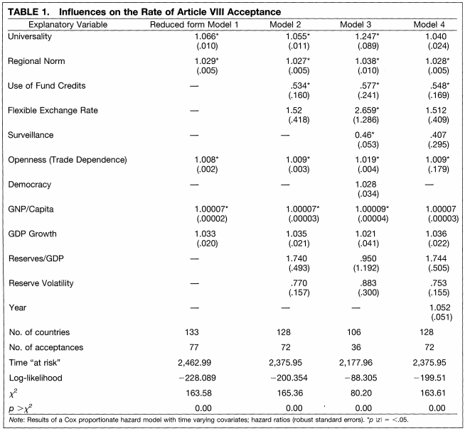
Example of Cox Proportional Hazards table from Simmons (2000)
14.3.1 Survival Models in R
We will do an example of these modeling approaches using the same package in R and dataset.
The workhorse of survival modeling is the Surv() function, which tells R the nature of your survival data, such as the duration variable and if the origin should be assumed to be 0 or if, instead, it is located under a different variable. The examples we use are very basic. If you are using this for your own research, I recommend investigating the options available in this function. The documentation is here.
14.3.2 Weibull Model
Note: survreg() fits what are called accelerated failure models, not proportional hazards models. The coefficients are logarithms of ratios of survival times, so a positive coefficient means longer survival. This is a different type of modeling specification than what other softwares, such as Stata, will default to when fitting the Weibull model. Both can be valid, but it matters for interpretation (what a positive vs. negative sign means in the model). Sarah Haile describes alternative ways to present these models using supplemental functions here.
wfit <- survreg(Surv(time=time, event=status)~ age + sex,
                data=lung,
                dist = "weibull")
summary(wfit)
Call:
survreg(formula = Surv(time = time, event = status) ~ age + sex,
    data = lung, dist = "weibull")
               Value Std. Error     z       p
(Intercept)  6.27485    0.48137 13.04 < 2e-16
age         -0.01226    0.00696 -1.76  0.0781
sex          0.38209    0.12748  3.00  0.0027
Log(scale)  -0.28230    0.06188 -4.56 5.1e-06

Scale= 0.754

Weibull distribution
Loglik(model)= -1147.1   Loglik(intercept only)= -1153.9
    Chisq= 13.59 on 2 degrees of freedom, p= 0.0011
Number of Newton-Raphson Iterations: 5
n= 228
We can interpret this as women having a higher survival duration than men. Positive coefficients for this model are associated with longer duration times. The hazard decreases and average survival time increases as the \(x\) covariate increases.
We can get different quantities of interest, such as a point at which 90% of patients survive.
# 90% of patients of these types survive past time point above
predict(wfit, type = "quantile", p =1-0.9,newdata =
          data.frame(age=65, sex=c(1,2)))
1 2
64.28587 94.20046 A survival curve can then be visualized as follows:
pct <- seq(.99, .01, by = -.01)
wb <- predict(wfit, type = "quantile", p =1-pct,newdata =
          data.frame(age=65, sex=1))

survwb <- data.frame(time = wb, surv = pct,
                      upper = NA, lower = NA, std.err = NA)
ggsurvplot(fit = survwb, surv.geom = geom_line,
           legend.labs="Male, 65")
14.3.3 Cox proportional Hazards Model
This model will rely on a different R function coxph(). Note the difference in interpretation.
fit <- coxph(Surv(time, status) ~ age  + sex,
             data = lung)
summary(fit)
Call:
coxph(formula = Surv(time, status) ~ age + sex, data = lung)
n= 228, number of events= 165
coef exp(coef) se(coef) z Pr(>|z|)
age 0.017045 1.017191 0.009223 1.848 0.06459 .
sex -0.513219 0.598566 0.167458 -3.065 0.00218 **
---
Signif. codes: 0 '***' 0.001 '**' 0.01 '*' 0.05 '.' 0.1 ' ' 1
exp(coef) exp(-coef) lower .95 upper .95
age 1.0172 0.9831 0.9990 1.0357
sex 0.5986 1.6707 0.4311 0.8311
Concordance= 0.603 (se = 0.025 )
Likelihood ratio test= 14.12 on 2 df, p=9e-04
Wald test = 13.47 on 2 df, p=0.001
Score (logrank) test = 13.72 on 2 df, p=0.001Here, positive coefficients mean that the hazard (risk of death) is higher.
- \(exp(\beta_k)\) is ratio of the hazards between two units where \(x_k\) differ by one unit.
- Hazard ratio above 1 is positively associated with event probability (death).
Visualizing Results
- The
survminerpackage has some shortcuts for this type of model. - A simple plot would be the overall survival probabilities from the model
library(ggplot2)
library(survminer)
cox1 <- survfit(fit)
ggsurvplot(cox1, data = lung)
We can also visualize the results by using the same types of approaches we do when we use the predict() function and specify new \(X\) data in other types of regression. Here, we will use the command survfit.
sex_df <- data.frame(sex = c(1,2), age = c(62, 62) )
cox1 <- survfit(fit, data = lung, newdata = sex_df)
ggsurvplot(cox1, data = lung, legend.labs=c("Sex=1", "Sex=2"))
You may wish to test the proportional hazards assumption. Here are two resources for this here and here.