12.3 Fixed Effects
In fixed effects, we allow the intercept to be different across our \(N\) groups (e.g., countries), where these terms are going to account for time-invariant (time constant) characteristics of these areas.
\[\begin{align*} Y_{it} &= \alpha_i + \beta_1x_{it} + \epsilon_{it} \end{align*}\]
where \(\alpha_{i}\) absorbs all unobserved time-invariant characteristics for unit \(i\) (e.g., features of geography, culture, etc.)
- This is huge! It’s going to help us get around the assumption we just talked about. The idea is that when we are comparing observations within a particular unit (e.g., within France), all of those time-invariant characteristics specific to France are held constant.
Below we discuss how to estimate fixed effects models. It is not the solution to everything. Keep these in mind.
- Still assume homoskedastic errors \(\rightarrow\) may want to adjust the SE’s.
- Cannot model “level-2” factors. Problematic if that’s what you’re interested in! (E.g., if you have time-invariant country-level covariates). Can only do this through interactions.
- For example, suppose we have a measure of a country’s culture (\(culture_{i}\)), that does not vary over time. We could not include that in our regression model because the model removes all time-invariant characteristics. In contrast, if something like country GDP changes a lot over time (\(GDP_{it}\)), it could still and should be accounted for.
- Only works if you have a decent number of observations
- Leverages within-group variation on your outcomes. Need to have this variation for it to make sense!
There are two general approaches for fitting fixed effects estimators: the within-estimator and LSDV.
12.3.1 Within-Estimator
Time Demeaning. First calculate averages of the \(it\) terms.
- Note, the mean of \(\alpha_i\) is just \(\alpha_i\) because it does not vary over time. \(\alpha_i\) because: \(\frac{1}{T} \sum_{t=1}^T \alpha_i = \frac{1}{T}*T*\alpha_i = \alpha_i\).
\[\begin{align*} \bar y_i &= \alpha_i + \beta\bar x_i + \bar \epsilon_i\\ \end{align*}\]
Subtracting we get: \[\begin{align*} Y_{it} - \bar y_i &= (\alpha_i -\alpha_i) + \beta(x_{it}- \bar x_i) + (\epsilon_{it}- \bar \epsilon_i)\\ \widetilde{Y_{it}} &= \beta\widetilde{x_{it}} + \widetilde{\epsilon_{it}} \end{align*}\] \(\beta\) is estimated just from deviations of the units from their means. Removes anything that is time-constant.
This video from Ben Lambert goes through the demeaning process.
12.3.2 Least Squares Dummy Variable Regression
We can estimate the equivalent model by including dummy variables in our regression. This is sometimes why you have seen authors add dummies for region and call them “fixed effects.”
OLS with dummy variables for each unit (e.g., countries). Start with “stacked” data where: \(Y = X\beta + U\delta + \epsilon\).
- \(Y\) is \(NT \times 1\) outcome vector where \(N\) is number of \(i\) units and \(T\) is number of time points \(t\).
- \(X\) is \(NT \times k\) matrix where \(k\) is the number of covariates plus general intercept
- \(U\) is a set of \(m\) dummy variables (e.g., country dummies), leaving one as reference
By accounting for these groups in our regression, we are now estimating how the covariates in \(\mathbf x\) affect our outcomes, holding constant the group– leveraging within-group variation.
12.3.3 Fixed Effects Implementation in R
The plm package allows us to indicate that our data are panel in nature and fit the within-estimator.
Run install.packages("plm") and load Grunfeld. 200 observations at the firm-year level. Here, we can think of firms as indexed by \(i\) and years indexed by \(t\).
library(plm)
data(Grunfeld)
head(Grunfeld)
firm year inv value capital
1 1 1935 317.6 3078.5 2.8
2 1 1936 391.8 4661.7 52.6
3 1 1937 410.6 5387.1 156.9
4 1 1938 257.7 2792.2 209.2
5 1 1939 330.8 4313.2 203.4
6 1 1940 461.2 4643.9 207.2## Unique N- firms
length(unique(Grunfeld$firm))[1] 10## Unique T- years
length(unique(Grunfeld$year))[1] 20For more detail onplm, see documentation
These data are used to study the effects of capital (stock of plant and equipment) on gross investment inv.
Let’s first run a standard OLS model, which we will call the “pooled” model because it pools observations across firms and years without explicitly accounting for them in the model. We can use the standard lm model to do this or the plm function from the plm package by indicating model="pooling". Both give equivalent results.
## Pooled model
fit.pool <- plm(inv~ capital, data = Grunfeld, model = "pooling")
coef(fit.pool)["capital"]
capital
0.4772241 ## Equivalent
fit.ols <- lm(inv~ capital, data = Grunfeld)
coef(fit.ols)["capital"] capital
0.4772241 We could visualize this model as follows by plotting the regression line. This provides a good benchmark against which we can see how fixed effects change the results. Note that the line ignores which firm that the data are coming from, using between-firm variation to help fit the regression slope.
library(ggplot2)
ggplot(Grunfeld, aes(x=capital, y=inv, color=as.factor(firm)))+
  geom_point()+
  geom_smooth(aes(y=inv), se=F, method="lm", color="black")
Let’s now fit our fixed effects model. Here, we have to add an argument that specifies which variables are indexed by \(i\) and \(t\) so that plm knows how to incorporate the individual firm units. We will first fit the within model using the plm package. We can then use lm by explicitly adding dummy variables. You will note that the individual dummy variable coefficients are only included in the output of lm and not plm. When you have a large number of units, it might be more computationally efficient and cleaner to use plm. However, both give us equivalent results for our coefficients of interest.
## Within model with firm fixed effects
fit.within <- plm(inv~capital,
                  data = Grunfeld,
                  model = "within",
                  index = c("firm", "year"))
coef(fit.within)["capital"]
capital
0.3707496 ## numerical equivalent
fit.lsdv <- lm(inv~ capital + as.factor(firm),
data = Grunfeld)
coef(fit.lsdv)["capital"] capital
0.3707496 Recall, what fixed effects does is create a different intercept by firm. We can visualize this by generating predicted gross investments for each observation in our data.
Fixed effects leverages within-firm variation to fit the regression model. That is, holding constant the firm, how does capital influence investment, on average?
Here, we see that when the variation is coming from within-firm, the estimated slope for the capital variable is slightly more shallow than when the pooled model used data across different firms to estimate the slope. Sometimes, the difference between the pooled OLS and fixed effects estimation can be so severe as to reverse the sign of the slopes. This is the idea of Simpson’s paradox discussed here.
fit.lsdvpred <- predict(fit.lsdv)
library(ggplot2)
ggplot(Grunfeld, aes(x=capital, y=inv, color=factor(firm)))+
  geom_point()+
  geom_smooth(aes(y=inv), se=F, method="lm", color="black")+
  geom_line(aes(y=fit.lsdvpred))
`geom_smooth()` using formula 'y ~ x'
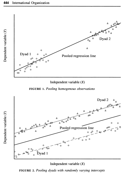
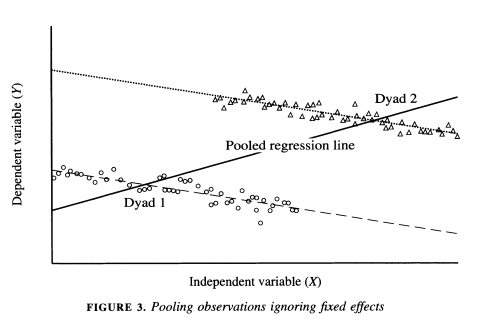
Green et al. (2003) also discuss the dangers of pooling data in certain cases in the article ``Dirty Pool.” Below are three examples. In the first two, pooling vs. fixed effects will not make much of a difference, but it will in the third.
As the authors describe, “The plot in Figure 1 depicts a positive relationship between X and Y where N = 2 and T = 50. Because both dyads share a common intercept, pooling creates no estimation problems. One obtains similar regression estimates regardless of whether one controls for fixed effects by introducing a dummy variable for each dyad. A pooled regression is preferable in this instance because it saves a degree of freedom. In Figure 2 we encounter another instance in which dyads have different intercepts, but there is no correlation between the intercepts and X. The average value of the independent variable is the same in each dyad. Again, pooled regression and regression with fixed effects give estimates with the same expected value. Figure 3 illustrates a situation in which pooled regression goes awry. Here, the causal relationship between X and Y is negative; in each dyad higher values of X coincide with lower values of Y. Yet when the dyads are pooled together, we obtain a spurious positive relationship. Because the dyad with higher values of X also has a higher intercept, ignoring fixed effects biases the regression line in the positive direction. Controlling for fixed effects, we correctly ascertain the true negative relationship between X and Y” (443-445).
12.3.4 Standard errors with fixed effects
Even if we use fixed effects, we may want to adjust standard errors. Fixed effects assumes homoskedasticity (constant error variance). We might instead think that the random error disturbances are correlated in some way or vary across time or units. For example, we might fear we have serial correlation (autocorrelation), where errors are correlated over time. Below are a few options.
Clustered standard errors. We came across this before in our section on ordinal probit models and the Paluck and Green paper. This blog post discusses why you may still want to cluster standard errors even if you have added fixed effects.
Note: the functions below are designed to work with the plm package and models. For models fit through other functions, you may need to use different functions to make adjustments. See section 8.5.1. For linear models lm_robust from the estimatr package works well. For other models, see the alternative applications in that section.
## Cluster robust standard errors to match stata (c only matters if G is small). Can omit if do not want to adjust for degrees of freedom.
## Generally want G to be 30 or 40
G <- length(unique(Grunfeld$firm))
c <- G/(G - 1)
sqrt(diag(c*vcovHC(fit.within,type = "HC1", cluster = "group")))
capital
0.06510863 Panel corrected SE: Beck and Katz have also developed standard errors for panel data. Explained in the documentation, observations may be clustered either by “group” to account for timewise heteroskedasticity and serial correlation or by “time” to account for cross-sectional heteroskedasticity and correlation. This is sensitive to \(N\) and \(T\).
## Alternative: Beck and Katz panel corrected standard errors
sqrt(diag(vcovBK(fit.within, cluster = "group"))) # also can change type
capital
0.04260805 Alternative: Adjusted for heteroskedasticity and/or serial correlation.
sqrt(diag(vcovHC(fit.within, type = "HC1", method = "arellano"))) capital
0.06176747 For more information, see pg. 24 of this resource