14.2 Kaplan-Meier Survival Function
A common way to summarize survival curves for actual data is through Kaplan-Meier curves.
This is a non-parametric analysis: Where \(n_j\) is the number of units at “risk” and \(d_j\) are the number of units failed at \(t_j\)
- For \(j: t_j \leq y\): \(S(\hat y) = \prod \frac{n_j - d_j}{n_j}\)
- Units surviving divided by unit at risk. Units that have died, dropped out, or not reached the time yet are not counted as at risk.
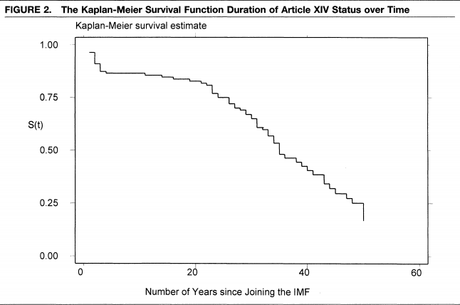
Example from Simmons (2000), “International law and state behavior: Commitment and compliance in international monetary affairs” published in the American Political Science Review.
- Note: unlike the nice theoretical parametric curve from above, often survival estimates from real data are more like “step functions.”
14.2.1 Kaplan-Meier in R
We will use the lung data from the survival package. For plotting, we will use the package survminer.
## install.packages("survival")
library(survival)
data("lung")
head(lung)
inst time status age sex ph.ecog ph.karno pat.karno meal.cal wt.loss
1 3 306 2 74 1 1 90 100 1175 NA
2 3 455 2 68 1 0 90 90 1225 15
3 3 1010 1 56 1 0 90 90 NA 15
4 5 210 2 57 1 1 90 60 1150 11
5 1 883 2 60 1 0 100 90 NA 0
6 12 1022 1 74 1 1 50 80 513 0time: days of survival.status: whether observation has failed or is right-censored. 1=censored, 2=dead.sex: Male=1; Female =2
Note: the place where we would normally put our outcome variable in a regression formula now takes Surv(time, event)
## Kaplan-Meier
sfit <- survfit(Surv(time=time, event=status)~sex, data=lung)

## install.packages("survminer")
library(survminer)
ggsurvplot(sfit,
           conf.int=TRUE,
           risk.table=TRUE,
           pval = TRUE,
           legend.labs=c("Male", "Female"),
           legend.title="Sex",
           title="Kaplan-Meier: for Lung Cancer Survival")