5.4 MLE Properties
Just like OLS had certain properties (BLUE) that made it worthwhile, models using MLE also have desirable features under certain assumptions and regularity conditions.
Large sample properties
- MLE is consistent: \(p\lim \hat \theta^{ML} = \theta\)
- It is also asymptotically normal: \(\hat \theta^{ML} \sim N(\theta, [I(\theta)]^{-1})\)
- This will allow us to use the normal approximation to calculate z-scores and p-values
- And it is asymptotically efficient. “In other words, compared to any other consistent and uniformly asymptotically Normal estimator, the ML estimator has a smaller asymptotic variance” (King 1998, 80).
Note on consistency
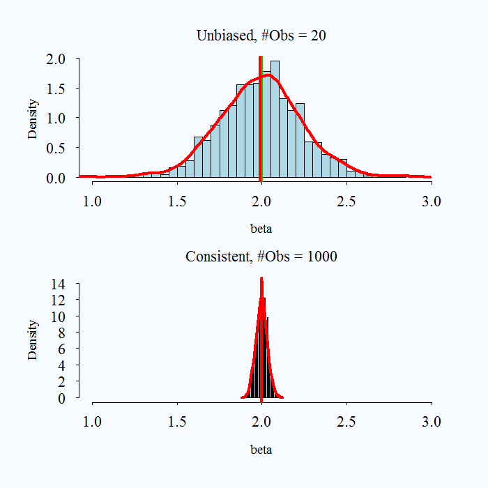
What does it mean to say an estimator is consistent? As samples get larger and larger, we converge to the truth.
Consistency: \(p\lim \hat{\theta} =\beta\) As \(n \rightarrow \infty P(\hat{\theta} - \theta> e) \rightarrow 0\).
- Convergence in probability: the probability that the absolute difference between the estimate and parameter being larger than \(e\) goes to zero as \(n\) gets bigger.
Note that bias and consistency are different: Consistency means that as the sample size (\(n\)) gets large the estimate gets closer to the true value. Unbiasedness is not affected by sample size. An estimate is unbiased if over repeated samples, its expected value (average) is the true parameter.
It is possible for an estimator to be unbiased and consistent, biased and not consistent, or consistent yet biased.
 ;
; 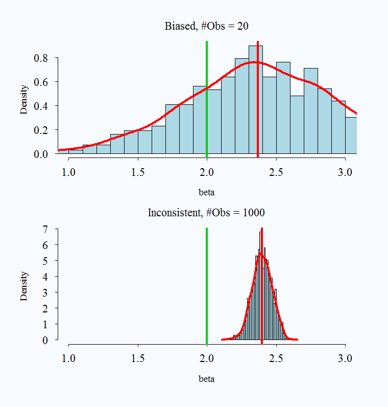

Images taken from here
What is a practical takeaway from this? The desirable properties of MLE kick in with larger samples. When you have a very small sample, you might use caution with your estimates.
No Free Lunch
We have hinted at some of the assumptions required, but below we can state them more formally.
- First, we assume a particular data generating process: the probability model.
- We are generally assuming that observations are independent and identically distributed (allowing us to write the likelihood as a product)– unless we explicitly write the likelihood in a way that takes this into account.
- When we have complicated structures to our data, this assumption may be violated, such as data that is clustered in particular hierarchical entities.
- We assume the model (i.e., the choice of covariates and how they are modeled) is correctly specified. (e.g., no omitted variables.)
- We have to meet certain technical regularity conditions–meaning that our problem is a “regular” one. These, in the words of Gary King are “obviously quite technical” (1998, 75). We will not get into the details, but you can see pg. 75 of Unifying Political Methodology for the formal mathematical statements. In short, our paramaters have to be identifiable and within the parameter space of possible values (this identifiability can be violated, for example, when we have too many parameters relative to the number of observations in the sample), we have to be able to differentiate the log-likelihood (in fact, it needs to be twice continuously differentiable) along the support (the range of values) in the data. The information matrix, which we get through the second derivative, must be positive definite and finitely bounded. This helps us know we are at a maximum, and the maximum exists and is finite. You can visualize this as a smooth function, that is not too sharp (which would make it non differentiable), but has a peak (a maximum) that we can identify.
5.4.1 Hypothesis Tests
We can apply the same hypothesis testing framework to our estimates here as we did in linear regression. First, we can standardize our coefficient estimates by dividing them by the standard error. This will generate a “z score.” Just like when we had the t value in OLS, we can use the z score to calculate the p-value and make assessments about the null hypothesis that a given \(\hat \beta_k\) = 0.
\[\begin{align*} z &= \frac{\hat \theta_k}{\sqrt{Var(\hat \theta)_k}} \sim N(0,1) \end{align*}\]
Note: to get p-values, we typically now use, 2 * pnorm(abs(z), lower.tail=F) instead of pt() and our critical values are based on qnorm() instead of qt(). R will follow the same in most circumstances. In large samples, these converge to the same quantities.
5.4.2 Model Output in R
As discussed, we can fit a GLM in R using the glm function:
glm(formula, data, family = XXX(link = "XXX", ...), ...)formula: The model written in the form similar tolm()data: Data framefamily: Name of PDF for \(Y_i\) (e.g.binomial,gaussian)link: Name of the link function (e.g.logit, `probit,identity,log)
## Load Data
fit.glm <- glm(participation ~ female + edu + age + sexism, data=anes,
               family=gaussian(link="identity"))
We’ve already discussed the coefficient output. Like lm(), GLM wiil also display the standard errors, z-scores / t-statistics, and p-values of the model in the model summary.
summary(fit.glm)$coefficients Estimate Std. Error t value Pr(>|t|)
(Intercept) 0.929302597 0.154033186 6.033132 1.999280e-09
female -0.217453631 0.067415200 -3.225588 1.282859e-03
edu 0.166837062 0.022402469 7.447262 1.559790e-13
age 0.008795138 0.001874559 4.691843 2.941204e-06
sexism -0.981808431 0.154664950 -6.347970 2.844067e-10For this example, R reverts to the t-value instead of the z-score given that we are using the linear model. In other examples, you may see z in place of t. There are only small differences in these approximations because as your sample size gets larger, the degrees of freedom (used in the calculation of p-calues for the t distribution) are big enough that the t distribution converges to the normal distribution.
Goodness of fit
The glm() model has a lot of summary output.
summary(fit.glm)
Call:
glm(formula = participation ~ female + edu + age + sexism, family = gaussian(link = "identity"),
    data = anes)

Deviance Residuals:
    Min       1Q   Median       3Q      Max
-2.3001  -0.8343  -0.3013   0.3651   7.2887

Coefficients:
             Estimate Std. Error t value Pr(>|t|)
(Intercept)  0.929303   0.154033   6.033 2.00e-09 ***
female      -0.217454   0.067415  -3.226  0.00128 **
edu          0.166837   0.022402   7.447 1.56e-13 ***
age          0.008795   0.001875   4.692 2.94e-06 ***
sexism      -0.981808   0.154665  -6.348 2.84e-10 ***
---
Signif. codes:  0 '***' 0.001 '**' 0.01 '*' 0.05 '.' 0.1 ' ' 1

(Dispersion parameter for gaussian family taken to be 1.688012)

    Null deviance: 2969.3  on 1584  degrees of freedom
Residual deviance: 2667.1  on 1580  degrees of freedom
AIC: 5334.9

Number of Fisher Scoring iterations: 2
Some of the output represents measures of the goodness of fit of the model. However, their values are not directly interpretable from a single model.
- Larger (less negative) likelihood, the better the model fits the data. (
logLik(mod)). The becomes relevant when comparing two or more models. - Deviance is calculated from the likelihood. This is a measure of discrepancy between observed and fitted values. (Smaller values, better fit.)
- Null deviance: how well the outcome is predicted by a model that includes only the intercept. (\(df = n - 1\))
- Residual deviance: how well the outcome is predicted by a model with our parameters. (\(df = n-k\))
- AIC- used for model comparison. Smaller values indicate a more parsimonious model. Accounts for the number of parameters (\(K\)) in the model (like Adjusted R-squared, but without the ease of interpretation). Sometimes used as a criteria in prediction exercises (using a model on training data to predict test data). For more information on how AIC can be used in prediction exercises, see here.
Likelihood Ratio Test
The likelihood ratio test compares the fit of two models, with the null hypothesis being that the full model does not add more explanatory power to the reduced model. Note: You should only compare models if they have the same number of observations.
This type of test is used in a similar way that people compare R-squared values across models.
fit.glm2 <- glm(participation ~ female + edu + age + sexism, data=anes,
               family=gaussian(link="identity"))

fit.glm1 <- glm(participation ~ female + edu + age, data=anes,
               family=gaussian(link = "identity"))

anova(fit.glm1, fit.glm2, test = "Chisq") #  reject the null
Analysis of Deviance Table
Model 1: participation ~ female + edu + age
Model 2: participation ~ female + edu + age + sexism
Resid. Df Resid. Dev Df Deviance Pr(>Chi)
1 1581 2735.1
2 1580 2667.1 1 68.021 2.182e-10 ***
---
Signif. codes: 0 '***' 0.001 '**' 0.01 '*' 0.05 '.' 0.1 ' ' 1Pseudo-R-squared
We don’t have an exact equivalent to the R-squared in OLS, but people have developed “pseudo” measures.
Example: McFadden’s R-squared
- \(PR^2 = 1 - \frac{\ell(M)}{\ell(N)}\)
- where \(\ell(M)\) is the log-likelihood for your fitted model and \(\ell(N)\) is the log-likelihood for a model with only the intercept
- Recall, greater (less negative) values of the log-likelihood indicate better fit
- McFadden’s values range from 0 to close to 1
# install.packages("pscl")
library(pscl)
Warning: package 'pscl' was built under R version 4.0.2Classes and Methods for R developed in the
Political Science Computational Laboratory
Department of Political Science
Stanford University
Simon Jackman
hurdle and zeroinfl functions by Achim Zeileisfit.glm.null <- glm(participation ~ 1, anes, family = gaussian(link = "identity"))
pr <- pR2(fit.glm1)fitting null model for pseudo-r2pr["McFadden"] McFadden
0.02370539 ## Or, by hand:
1 - (logLik(fit.glm1)/logLik(fit.glm.null))'log Lik.' 0.02370539 (df=5)