8.1 Ordinal Outcome Data

Here is a motivating example for the use of ordered data from Paluck and Green “Deference, Dissent, and Dispute Resolution: An Experimental Intervention Using Mass Media to Change Norms and Behavior in Rwanda” which was published in the American Political Science Review in 2009. doi:10.1017/S0003055409990128

Abstract. Deference and dissent strike a delicate balance in any polity. Insufficient deference to authority may incapacitate government, whereas too much may allow leaders to orchestrate mass violence. Although cross-national and cross-temporal variation in deference to authority and willingness to express dissent has long been studied in political science, rarely have scholars studied programs designed to change these aspects of political culture. This study, situated in post-genocide Rwanda, reports a qualitative and quantitative assessment of one such attempt, a radio program aimed at discouraging blind obedience and reliance on direction from authorities and promoting independent thought and collective action in problem solving. Over the course of one year, this radio program or a comparable program dealing with HIV was randomly presented to pairs of communities, including communities of genocide survivors, Twa people, and imprisoned genocidaires … Although the radio program had little effect on many kinds of beliefs and attitudes, it had a substantial impact on listeners’ willingness to express dissent and the ways they resolved communal problems.

In a field experiment, the authors have randomly assigned participants in different research sites to listen to a radio program over the course of a year that varied in its message. As the authors note, “Because radios and batteries are relatively expensive for Rwandans, they usually listen to the radio in groups. Thus, we used a group-randomized design in which adults from a community listened together either to the treatment (reconciliation) program or to the control program (another entertainment-education radio soap opera about health and HIV).” The authors have 14 clusters without 40 individuals within each cluster.

Treatment (treat): radio program with one of two messages, where 1=the treatment condition with a reconciliation message and 0=control, listening to a health message.
Outcome (dissent): Willingness to Display Dissent: An ordered scale with four categories from 1 (“I should stay quiet”) to 4 (“I should dissent”)

Let’s load the data and look at the treatment and outcome.

library(rio)
pg <- import("https://github.com/ktmccabe/teachingdata/blob/main/paluckgreen.dta?raw=true")

## Let's treat the outcome as a factor
pg$dissent <- as.factor(pg$dissent)

## Let's visualize the outcome by group
library(ggplot2)
library(tidyverse)
pg %>%
  filter(is.na(dissent)==F) %>%
  ggplot(aes(x=dissent, group=factor(treat), 
               fill=factor(treat)))+
  geom_bar(aes(y=..prop..),stat= "count", position="dodge", color="black")+
  theme_minimal()+
  theme(legend.position = "bottom")+
  scale_fill_brewer("Condition", labels=c("Control", "Treatment"),palette="Paired")+
  scale_x_discrete(labels= c("Should Stay Quiet", "2", "3", "Should Dissent"))

We can see variation in the outcome, where some people are at the “stay quiet” end of the scale, while others are at the opposite end. We might have a few questions about the outcome:

What is the probability of being in a particular category given a set of \(\mathbf{x_i'}\) values?
Does the treatment influence likelihood of expressing dissent?
Does the treatment significantly affect the probability of responding in a particular category?

What model should they use to help answer these questions?

One approach would be to use OLS.

They could treat 1 to 4 scale as continuous from Should stay quiet to Should dissent
If they do this, the interpretation of the regression coefficients would be:
- Going from Control to Treatment (0 to 1), is associated with \(\hat \beta\) movement on this scale.
What could be problematic here?
- Might go below or above scale points
- Distance between scale points might not be an equal interval
- Doesn’t answer the “probability” question, just describes movement up and down the scale.

A second approach could be to collapse the scale to be dichotomous and use logit/probit or a linear probability model.

For example, they could treat the outcome to 0 = (lean toward stay quiet/stay quiet) vs. 1 (lean toward dissent/dissent)
Here, after converting the outcomes in probability, the interpretation would be
- Going from Control to Treatment (0 to 1), is associated with an average difference in predicted probability of dissent (\(Y_i = 1\))
What could be problematic here?
- We lose information.

A third approach–and the focus of this section– would be to use an ordinal logistic or probit regression.

This is appropriate when our goal, at least in part, is to estimate the probability of being in a specific category, and these categories have a natural ordering to them.

8.1.1 Ordinal Model

With ordered data, we have an outcome variable \(Y_i\) that can fall into different, ordered categories: \(Y_i \in \{C_1, C_2, \ldots, C_J \}\) with some probability.

The image above shows a distribution where the area under the curve sums to 1, with the area divided into 4 categories, separated by three cutpoints. The area represents probability mass. For example, the area to the left of z1 represents the \(Pr(Y_i^\ast \leq z1)\).

In our ordered model, we assume that there is a latent (unobserved) \(Y^\ast_i = X_i\beta + \epsilon\)

This means we can still have a single model \(X_i \beta\), which determines what outcome level is achieved (this requires an assumption).
where \(\epsilon\) is either assumed to be normally distributed (probit) or distributed logistically (logit), and corresponds to the fuzziness of the cutpoints (\(\zeta_j\)), which define in which category an outcome is observed to fall. Instead of fine lines, we estimate probabilistically in which category \(Y_i\) is predicted to fall.

We observe this category in our outcome: \(Y_i\).

For example, we observe if someone said “should stay quiet” or “should dissent” vs. one of the two middle categories.

\[\begin{gather*} Y_i=\begin{cases} C_1 \textrm{ if } Y^\ast_i \le \zeta_1\\ C_2 \textrm{ if } \zeta_1 < Y^\ast_i \le \zeta_2\\ C_3 \textrm{ if } \zeta_2 < Y^\ast_i \le \zeta_3\\ \ldots\\ C_J\textrm{ if } \zeta_{J-1} < Y^\ast_i \\ \end{cases}\\ \end{gather*}\]

The \(\zeta_j\) are called “cutpoints”

Need cutpoints that are distinct, but the distance between cutpoints does not have to be the same.
- This can be particularly useful when we have scales that have a natural ordering, but the distance between scale points might not have the same meaning or be the same (e.g., “Agree”,“Disagree”, “Revolt”). This is different from an interval variable, where we assume the difference between scale points carries the same meaning (e.g., credit score, cups of flour in a recipe).
Note: There is no intercept in linear prediction model in this case. Instead of the intercept, we have the specific cutpoints.
Rule of thumb: Estimation with more than 3-5 categories unstable

8.1.2 Interpretation

Here is an example of what the ordered probit model output can look like from the authors’ paper. You can see coefficients similar to the models we’ve been working with before but instead of an intercept, we have the different cutpoints, in this case, three cutpoints for \(J-1\) categories.

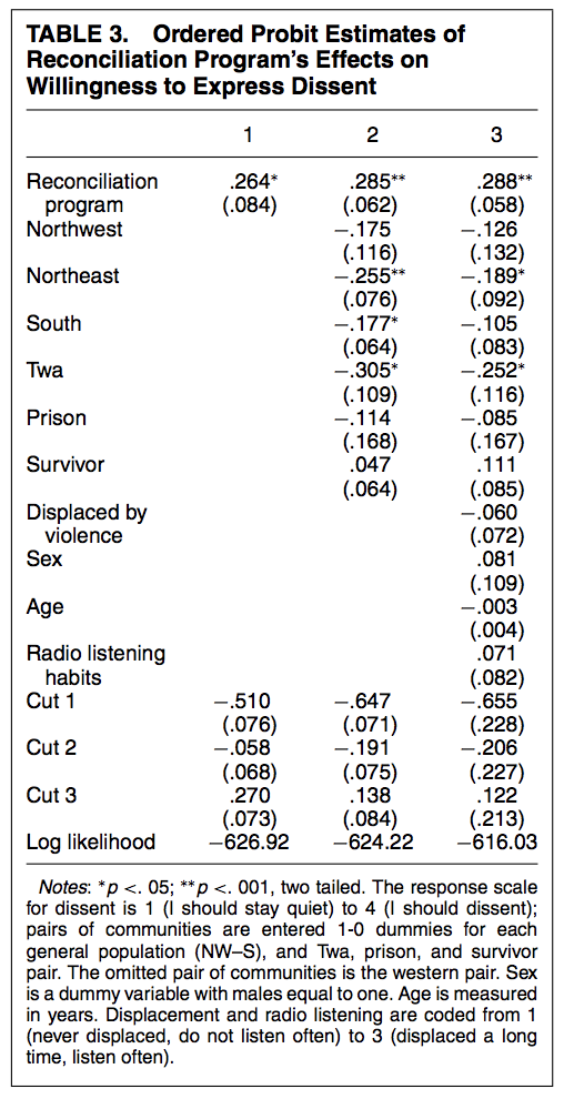
We can interpret the coefficients as a one-unit increase in \(x\) has a \(\hat \beta\) increase/decrease in the linear predictor scale of \(Y^\ast\) (in log-odds for logit or probit z-score standard deviations).

This gives us an initial sense (based on sign and significance) of how an independent variable positively or negatively affects the position of \(Y*\). However, it does not give us any information about specific categories.
Thus, alas, this is unsatisfying for a couple of reasons.
- \(Y_i^\ast\) is an unobserved variable (not the categories themselves)
- The scale is harder to interpret than probability
Therefore, we will generally want to convert our estimates into probabilities (our quantities of interest)
- One wrinkle here is we now have \(J\) predicted probabilities to estimate, one for each category.
- A second wrinkle here is any change in the probability of being in the \(jth\) category of \(Y\) also affects the probabilities of being in the \(\neq jth\) categories because the probabilities of being in each category have to sum together to 1. (E.g., Increasing the probability that someone said “should dissent” affects the probability they said “should stay quiet.)