8.5 Ordinal Practice Problems

Here are a few practice problems for ordered models.

1. Try to replicate column 2 from Table 3 by adding factor(site_pr) to the regression model. Note that the standard errors will not exactly match. We will discuss why in a follow-up section.
2. Calculate the average predicted probability of leaning toward staying quiet (category 2) for the treatment and control group, holding covariates at observed values.
   • Note: If you do this manually, you need to remove the intercept column that is automatically added to the model.matrix

Try on your own, and then expand for the solution.

fit.c2 <- polr(as.factor(dissent) ~ treat + factor(site_pr), 
               data=pg, method="probit", Hess =T)
coef(fit.c2)

           treat factor(site_pr)2 factor(site_pr)3 factor(site_pr)4 
      0.28484306      -0.17480464      -0.25513562      -0.17731799 
factor(site_pr)5 factor(site_pr)6 factor(site_pr)7 
     -0.30547159      -0.11384681       0.04659582 

## Option 1
library(prediction)
p1 <- prediction(fit.c2, at=list(treat=c(0,1)), category=2)
summary(p1)$Prediction

[1] 0.1726136 0.1537839

## Option 2
X <- model.matrix(fit.c2)[,-1]
X[, "treat"]<-1
bh <- coef(fit.c2)
eta <- X %*% bh
cutpoint2 <- fit.c2$zeta[2]
cutpoint1 <- fit.c2$zeta[1]
mean(pnorm(cutpoint2 - eta) - pnorm(cutpoint1 - eta))

[1] 0.1537839

X[, "treat"] <-0
bh <- coef(fit.c2)
eta <- X %*% bh
cutpoint2 <- fit.c2$zeta[2]
cutpoint1 <- fit.c2$zeta[1]
mean(pnorm(cutpoint2 - eta) - pnorm(cutpoint1 - eta))

[1] 0.1726136

8.5.1 A note on robust standard errors

In writing down our likelihood equations, we assume our observations are independent. However, that is not always the case. For example, in Paluck and Green’s article, the experimental design is based on clustered pairs, and the treatment is randomly assigned to one unit of a pair. Ideally, we want to account for this non-independence in our model.

In linear models (e.g., using lm), this is often accomplished post-estimation by adjusting the standard errors. We might adjust them for clustering if we have a case like the authors’ or for suspected heteroskedasticity (maybe the errors are not constant, but instead, are larger for higher values of a given X variable).

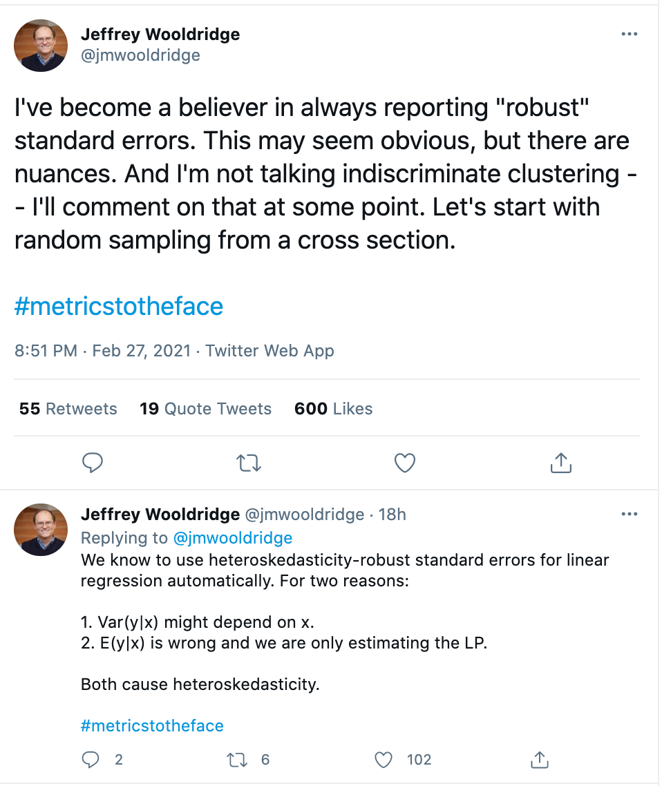
Professor Jeffrey Wooldridge, an expert on econometrics, is a proponent of robust standard errors, given the stringent assumption of homoskedasticity.

There are many types of these “robust” standard errors, and we may encounter more later in the course. Generally, what each of these robust standard errors does is alter the nature of the variance covariance matrix from which we extract the standard errors. Recall in OLS, we have an expression for the variance of the coefficients that looks like the below. By assuming constant error variance, we can simplify it.

\[\begin{align*} \mathbf{V}(\widehat{\beta}) &= (X^T X)^{-1}X^T \mathbf{V}( \epsilon) X (X^T X)^{-1}\\ &= \underbrace{(X^T X)^{-1}X^T \sigma^2I_n X (X^T X)^{-1}}_\text{Assume homoskedasticity}\\ &= \underbrace{\sigma^2(X^T X)^{-1} X^T X (X^T X)^{-1}}_\text{Because it is a constant, we can move it out in front of the matrix multiplication, and then simplify the terms.} \\ &= \sigma^2(X^T X)^{-1} \end{align*}\]

After we plug in \(\hat \sigma^2\) for \(\sigma^2\), we arrive at our variance-covariance matrix vcov:\(\hat \sigma^2(X^T X)^{-1}=\frac{1}{N-K} \mathbf{e'e}(X^T X)^{-1}\)

When we don’t have constant error variance, we have to pause here:

\((X^T X)^{-1}X^T \mathbf{V}( \epsilon) X (X^T X)^{-1}\)

and assume something different about the structure of the error terms in \(\mathbf{V}( \epsilon)\) and end up with a different final expression for vcov.

The robust estimators differ in how they specify an estimate for \(\mathbf{V}( \epsilon) = \Sigma\) and whether they take into account the degrees of freedom in the model (number of observations, number of variables, number of clusters, etc.)

For example, let’s fit the authors’ model as a linear model using MacKinnon and White HC1 robust standard errors. Those specify the following inside portion for an estimate of \(\mathbf{V}( \epsilon)\).This is what Stata uses as a default “robust” standard error:

\(\Sigma = \frac{n}{n-k} \text{diag}(\hat \epsilon_i^2)\)

This means we have a slightly different term for each observation instead of a constant estimate \(\hat \sigma^2\) for all observations.

fit.lin <- lm(as.numeric(dissent) ~ treat + factor(site_pr), 
               data=pg)

## Option 1: Adjusting for heteroskedasticity
library(sandwich)
newvcov <- vcovHC(fit.lin, type="HC1")
sqrt(diag(newvcov))

     (Intercept)            treat factor(site_pr)2 factor(site_pr)3 
       0.1661596        0.1145570        0.2128812        0.2158906 
factor(site_pr)4 factor(site_pr)5 factor(site_pr)6 factor(site_pr)7 
       0.2164289        0.2176110        0.2175578        0.2085747 

## Option 2: Adjusting for heteroskedasticity
library(estimatr)
fit.lin2 <- lm_robust(as.numeric(dissent) ~ treat + factor(site_pr), 
               data=pg, se_type = "stata")
sqrt(diag(vcov(fit.lin2)))

     (Intercept)            treat factor(site_pr)2 factor(site_pr)3 
       0.1661596        0.1145570        0.2128812        0.2158906 
factor(site_pr)4 factor(site_pr)5 factor(site_pr)6 factor(site_pr)7 
       0.2164289        0.2176110        0.2175578        0.2085747 

Another adjustment takes into account the grouped or “clustered” nature of the data. Here, we have a separate estimate for each group in the data. This can be implemented in R by using vcovCL or the clusters argument in lm_robust.

## Option 1: Adjusting for clustering
library(sandwich)
newvcov <- vcovCL(fit.lin, type="HC1", cadjust=T, cluster = pg$sitcode)
sqrt(diag(newvcov))

     (Intercept)            treat factor(site_pr)2 factor(site_pr)3 
      0.07685775       0.07066623       0.12388030       0.09271341 
factor(site_pr)4 factor(site_pr)5 factor(site_pr)6 factor(site_pr)7 
      0.07174477       0.12894245       0.20605985       0.06962861 

## Option 2: Adjusting for clustering
library(estimatr)
fit.lin2 <- lm_robust(as.numeric(dissent) ~ treat + factor(site_pr), 
               data=pg, se_type = "stata", clusters = sitcode)
sqrt(diag(vcov(fit.lin2)))

     (Intercept)            treat factor(site_pr)2 factor(site_pr)3 
      0.07685775       0.07066623       0.12388030       0.09271341 
factor(site_pr)4 factor(site_pr)5 factor(site_pr)6 factor(site_pr)7 
      0.07174477       0.12894245       0.20605985       0.06962861 

This is all great, but the authors don’t have a linear model, they have an ordered probit model. It turns out that people have developed similar robust standard error estimators to adjust the standard errors from these non-linear models. For more details, see slides from Molly Roberts on this point.

These take a slightly different form, but the intuition is the same. What we are altering is the structure of the variance-covariance matrix (which is a function of the Hessian in the likelihood case), making adjustments across all observations or clusters of observations.

We can also implement these in R using HC0 standard errors.

## Adjusting for clustered standard errors
fit.c2 <- polr(as.factor(dissent) ~ treat + factor(site_pr), 
               data=pg, method="probit", Hess =T)
clval <- vcovCL(fit.c2, type="HC0", cluster = pg$sitcode)

You can compare these standard errors to column 2 from Table 3 in the paper.

sqrt(diag(clval))

           treat factor(site_pr)2 factor(site_pr)3 factor(site_pr)4 
      0.06212521       0.11636326       0.07559847       0.06387804 
factor(site_pr)5 factor(site_pr)6 factor(site_pr)7              1|2 
      0.10879657       0.16765260       0.06391195       0.07144512 
             2|3              3|4 
      0.07494704       0.08409084 

The coeftest function in R, when applied to a new vcov will reproduce the full regression output.

library(lmtest)
coeftest(fit.c2, vcov=clval)

z test of coefficients:

                  Estimate Std. Error z value  Pr(>|z|)    
treat             0.284843   0.062125  4.5850  4.54e-06 ***
factor(site_pr)2 -0.174805   0.116363 -1.5022 0.1330371    
factor(site_pr)3 -0.255136   0.075598 -3.3749 0.0007385 ***
factor(site_pr)4 -0.177318   0.063878 -2.7759 0.0055052 ** 
factor(site_pr)5 -0.305472   0.108797 -2.8077 0.0049892 ** 
factor(site_pr)6 -0.113847   0.167653 -0.6791 0.4970975    
factor(site_pr)7  0.046596   0.063912  0.7291 0.4659633    
1|2              -0.646720   0.071445 -9.0520 < 2.2e-16 ***
2|3              -0.190723   0.074947 -2.5448 0.0109348 *  
3|4               0.138053   0.084091  1.6417 0.1006487    
---
Signif. codes:  0 '***' 0.001 '**' 0.01 '*' 0.05 '.' 0.1 ' ' 1

I got 99 problems, and standard errors are just one

However, robust standard errors cannot correct underlying model misspecification. Recall that the initial likelihood equation is what assumes independence– this is the equation we use for everything, not only for computing standard errors but also for estimating the coefficients themselves. If we truly believe we have dependence among our observations, we might consider using an entirely different likelihood function– one that incorporates this dependence, instead of just adjusting the standard errors after the fact.

Nonetheless, we may still think our model is good enough, even if not “correct.” So long as you recognize that the robust standard errors don’t correct for this underlying problem, some are still proponents for using robust standard errors in these cases. For example, Wooldridge recommends reporting robust standard errors, and writes,