6.4 To logit or to probit?

Both approaches produce a monotonically increasing S-curve in probability between 0 and 1, which vary according to the linear predictor (\(\mathbf{x_i}^T\beta\)). In this way, either approach satisfies the need to keep our estimates, when transformed, within the plausible range of \(Y\).

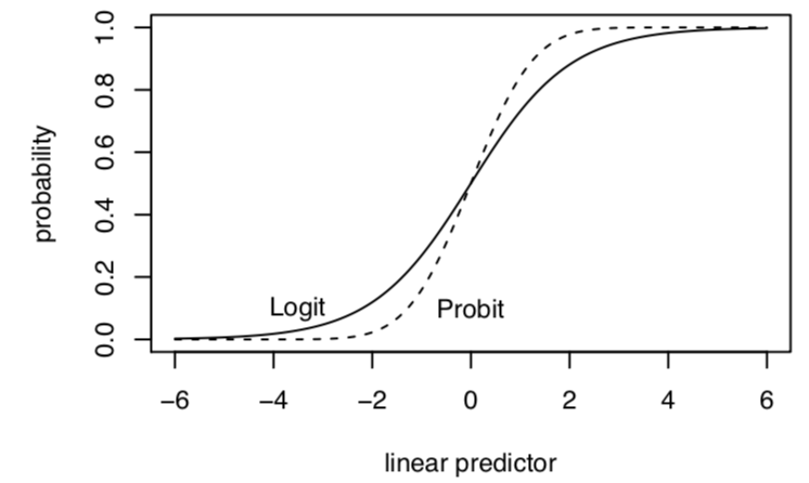Image from Kosuke Imai.

• Both also start with \(Y_i\) as bernoulli
• Both produce the same function of the log-likelihood BUT define \(\pi_i\) and link function differently
• Results–in terms of sign and significance of coefficients– are very similar
  • Logit coefficients are roughly 1.6*probit coefficients
• Results–in terms of predicted probabilities– are very similar
  • Exception– at extreme probabilities– Logit has “thicker tails”, gets to 0 and 1 more slowly
• Sometimes useful–Logit can also be transformed into “odds ratios”
• By convention, logit slightly more typically used in political science but easy enough to find examples of either

Note on Odds Ratios in Logistic Regression

Coefficients are in “logits” or changes in “log-odds” (\(\log \frac{\pi_i}{1 - \pi}\)). Some disciplines like to report “odds ratios”

• Odds ratio: \(\frac{\pi_i(x1)/(1 - \pi(x1))}{\pi_i(x0)/(1 - \pi(x0))}\) (at a value of x1 vs. x0)
  • If \(\log \frac{\pi_i}{1 - \pi} = logodds\); \(\exp(logodds) = \frac{\pi_i}{1 - \pi}\)
  • Therefore, if we exponentiate our coefficients, this represents an odds ratio: the odds of \(Y_i = 1\) increase by a factor of (\(\exp(\hat \beta_k)\)) due to 1-unit change in X

## odds ratio for the 4th coefficient
exp(coef(out.logit)[4])

    age 
1.00872 

## CI for odds ratios
exp(confint(out.logit)[4, ])

Waiting for profiling to be done...

   2.5 %   97.5 % 
1.000790 1.016801 

In political science, we usually opt to present predicted probabilities instead of odds ratios, but ultimately you should do whatever you think is best.