10.5 Quasipoisson and Negative Binomial Models
The quaipoisson model relaxes the assumption that the mean and variance have to be equivalent. It is the same as the Poisson but multiplies the standard errors by \(\sqrt{d}\), where \(d\) is the dispersion parameter.
These models are fit in R almost exactly the same way as poisson. We just switch family = "quasipoisson"
- Note in the
summaryoutput, it lists the dispersion parameter.
fitq <- glm(allnoncerm_eo ~ divided + inflation + spending_percent_gdp
            + war + lame_duck +
                 administration_change + trend +
            + tr+ taft + wilson + harding
           + coolidge + hoover,
           family = "quasipoisson",
           data = subset(bolton, year < 1945))
summary(fitq)
Call:
glm(formula = allnoncerm_eo ~ divided + inflation + spending_percent_gdp +
    war + lame_duck + administration_change + trend + +tr + taft +
    wilson + harding + coolidge + hoover, family = "quasipoisson",
    data = subset(bolton, year < 1945))

Deviance Residuals:
    Min       1Q   Median       3Q      Max
-8.2027  -2.4224  -0.1515   2.1532   8.9032

Coefficients:
                        Estimate Std. Error t value Pr(>|t|)
(Intercept)            8.0360573  0.9848054   8.160 1.22e-08 ***
divided                0.4435893  0.1727719   2.567  0.01634 *
inflation              0.0005599  0.0110836   0.051  0.96010
spending_percent_gdp  -0.0286140  0.0082874  -3.453  0.00191 **
war                    0.4745189  0.1936737   2.450  0.02133 *
lame_duck              0.3692336  0.2769252   1.333  0.19399
administration_change -0.0321975  0.1844677  -0.175  0.86279
trend                 -0.0619311  0.0316454  -1.957  0.06116 .
tr                    -2.5190839  0.9562064  -2.634  0.01401 *
taft                  -2.4104113  0.8805222  -2.737  0.01102 *
wilson                -1.4750129  0.6866621  -2.148  0.04120 *
harding               -1.4205088  0.4700492  -3.022  0.00558 **
coolidge              -1.1070363  0.3792082  -2.919  0.00715 **
hoover                -0.9985352  0.3099077  -3.222  0.00341 **
---
Signif. codes:  0 '***' 0.001 '**' 0.01 '*' 0.05 '.' 0.1 ' ' 1

(Dispersion parameter for quasipoisson family taken to be 16.96148)

    Null deviance: 1281.92  on 39  degrees of freedom
Residual deviance:  439.87  on 26  degrees of freedom
AIC: NA

Number of Fisher Scoring iterations: 4
The dispersion parameter is estimated using those standardized residuals from the Poisson model.
sres <- residuals(fit, type="pearson")
chisq <- sum(sres^2)
d <- chisq/fit$df.residual
d
[1] 16.96146Let’s compare the Poisson and Quasipoisson model coefficients and standard errors.
round(summary(fit)$coefficients[2,], digits=4) Estimate Std. Error z value Pr(>|z|)
0.4436 0.0420 10.5740 0.0000 round(summary(fitq)$coefficients[2,], digits=4) Estimate Std. Error t value Pr(>|t|)
0.4436 0.1728 2.5675 0.0163 We can retrieve the standard error from the quasipoisson by multiplication.
## Multiply the Poisson standard error by sqrt(d)
round(summary(fit)$coefficients[2,2] * sqrt(d), digits=4)
[1] 0.1728Note that the standard error among the Quasipoisson model is much bigger, accounting for the larger variance from overdispersion.
10.5.1 Negative Binomial Models
Another model commonly used for count data is the negative binomial model. This is the model Bolton and Thrower use. This has a more complicated likelihood function, but, like the quasipoisson, it has a larger (generally, more correct) variance term. Analogous to the normal distribution, the negative binomial has both a mean and variance term parameter.
\(\Pr(Y=y) = \frac{\Gamma(r+y)}{\Gamma(r) \Gamma(y+1)} (\frac{r}{r+\lambda})^r (\frac{\lambda}{r+\lambda})^y\)
- Models dispersion through term \(r\)
- \(\mathbf E(Y_i|X) = \lambda_i = e^{\mathbf x_i^\top \beta}\)
- \(\mathbf Var(Y_i|X) = \lambda_i + \lambda_i^2/r\) (note, this is no longer just \(\lambda_i\))
Note that while the probability distribution looks much uglier, the mapping of \(\mathbf x_i' \beta\) is the same. We will still have a \(\log\) link and exponeniate to get our quantities of interest. The mechanics work essentially the same as the poisson.
In R, we use the glm.nb function from the MASS package to fit negative binomial models. Here, we do not need to specify a family, but we do specify the link = "log".
library(MASS)
fitn <- glm.nb(allnoncerm_eo ~ divided + inflation +
                 spending_percent_gdp + war + lame_duck +
                 administration_change + trend +
            + tr+ taft + wilson + harding
           + coolidge + hoover,
           link="log",
           data = subset(bolton, year < 1945))
summary(fitn)$coefficients[2,]
Estimate Std. Error z value Pr(>|z|)
0.442135921 0.141831942 3.117322607 0.001825017 Compare this to column 1 in the model below.
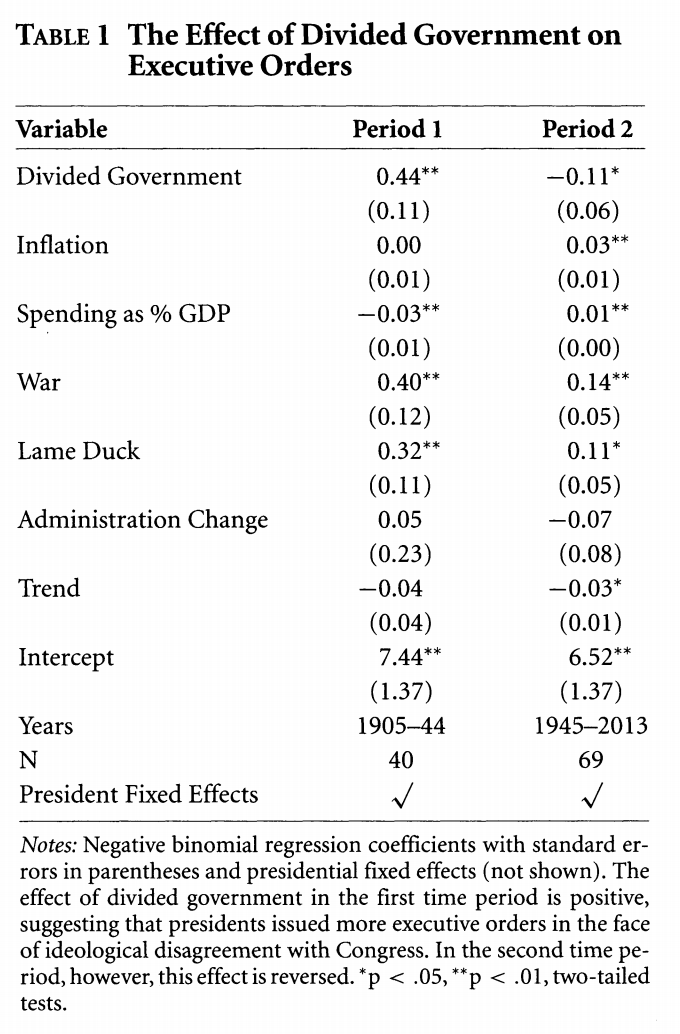
We have now replicated the coefficients in column 1 of Table 1 in the authors’ paper. Our standard errors do not match exactly because the authors use clustered standard errors by president. Moreover, given a relatively small sample the two programs R (and Stata, which the authors use) might generate slightly different estimates.