7.7 Putting everything together

Recall, we can take something that looks like column 5 in the table from Antoine Banks and Heather Hicks example from the previous section and move it into a figure, as the authors did.

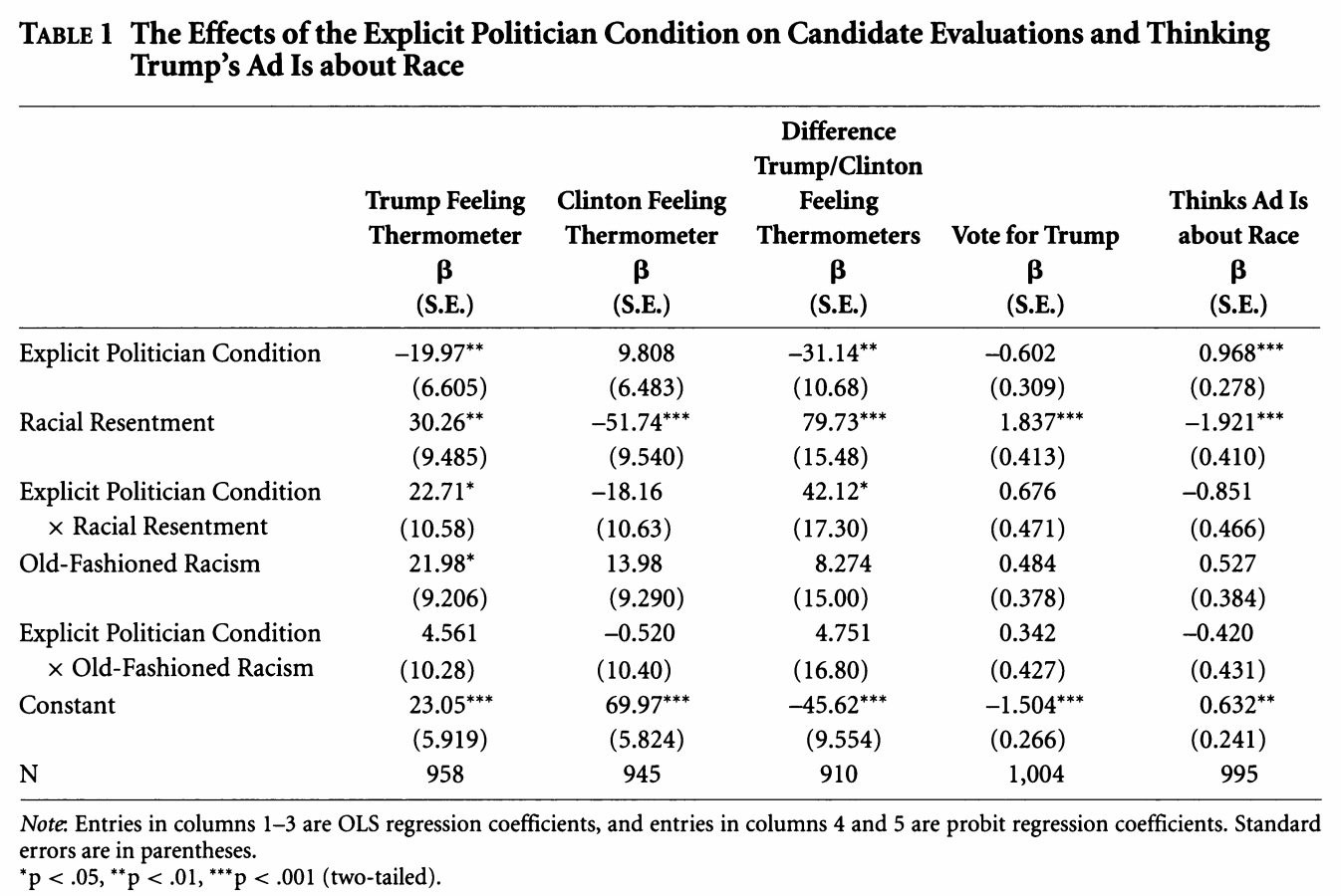
Let’s run the model from column 5.

fit.probit5 <- glm(abtrace1 ~ factor(condition2)*racresent 
                   + factor(condition2)*oldfash,
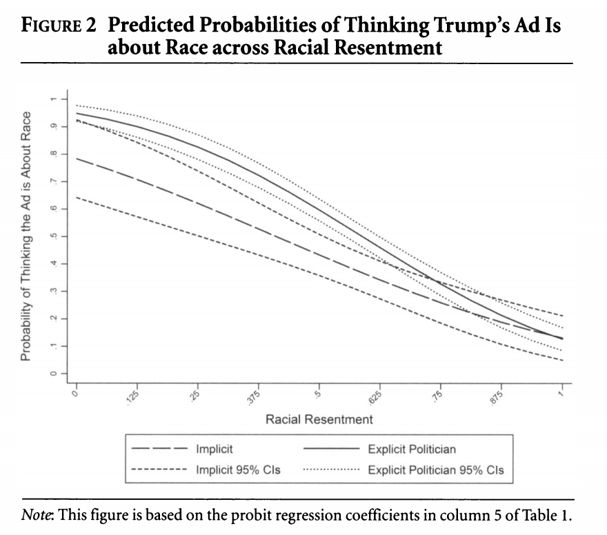
                  data=study, family=binomial(link = "probit"))

Let’s generate predicted probabilities for thinking the ad is about race across levels of racial resentment in the sample, for people in the implicit and explicit conditions, holding all covariates at observed values.

library(prediction)
pr.imp <- prediction(fit.probit5, at= list(racresent = seq(0, 1,.0625),
                                               condition2=1),
                         calculate_se = TRUE)
## Let's store the summary output this time
## And to make it easier to plot, we'll store as dataframe
pr.imp.df <- summary(pr.imp)

pr.exp <- prediction(fit.probit5, at= list(racresent = seq(0, 1,.0625),
                                               condition2=2),
                         calculate_se = TRUE)
pr.exp.df <- summary(pr.exp)

You can peek inside pr.imp.df to see the format of the output.

Let’s now visualize! We will try to stay true to the authors’ visual choices here.

## Plot results
plot(x=pr.imp.df$`at(racresent)`, y=pr.imp.df$Prediction, 
     type="l",
     ylim = c(0, 1), lty=2,
     ylab = "Predicted Probability",
     xlab = "Racial Resentment",
     main = "Predicted Probability of Viewing the Ad as about Race",
     cex.main = .7)
## add explicit point values
points(x=pr.exp.df$`at(racresent)`, y=pr.exp.df$Prediction, type="l")

## add additional lines for the upper and lower confidence intervals
points(x=pr.exp.df$`at(racresent)`, y=pr.exp.df$lower, type="l", col="gray")
points(x=pr.exp.df$`at(racresent)`, y=pr.exp.df$upper, type="l", col="gray")

points(x=pr.imp.df$`at(racresent)`, y=pr.imp.df$lower, type="l", lty=3)
points(x=pr.imp.df$`at(racresent)`, y=pr.imp.df$upper, type="l", lty=3)

## Legend
legend("bottomleft", lty= c(2,1, 3,1), 
       c("Implicit", "Explicit", 
         "Implicit 95% CI", "Explicit 95% CI"), cex=.7)

Let’s combine the two dataframes.

pr.comb <- rbind(pr.imp.df, pr.exp.df)

library(ggplot2)
ggplot(pr.comb, aes(x=`at(racresent)`, 
                    y= Prediction, 
                    color=as.factor(`at(condition2)`)))+
  geom_line()+
  geom_ribbon(aes(ymin=lower, ymax=upper, fill=as.factor(`at(condition2)`)), alpha=.5)+
  xlab("Racial Resentment")+
  theme_bw()+
  theme(legend.position = "bottom") +
  scale_color_discrete(name="Condition",
                         breaks=c(1,2),
                         labels=c("Implicit", "Explicit"))+
  scale_fill_discrete(name="Condition",
                         breaks=c(1,2),
                         labels=c("Implicit", "Explicit"))

We could instead show the difference between the conditions across levels of racial resentment.

library(margins)
marest <- margins(fit.probit5, at= list(racresent = seq(0, 1,.0625)),
                  variables="condition2",
                  change = c(1,2),
                         vce="delta",
                  type="response")

## Store summary as dataframe
marest.df <- summary(marest)

## plot res
ggplot(marest.df, aes(x=racresent, y=AME))+
  geom_line()+
  geom_errorbar(aes(ymin=lower, ymax=upper), alpha=.5, width=0)+
  theme_bw()+
  xlab("Racial Resentment")+
  ggtitle("AME: Explicit - Implicit Condition on Pr(Ad About Race)")+
  geom_hline(yintercept = 0, color="red")