1 Introduction

1.1 What have I signed up for?

First: What is Data Science?

Data Science involves a combination of math/statistics and programming/coding skills, which, for our purposes, we will combine with social science knowledge.
- Drew Conway has a nice venn diagram of how these different skill sets intersect.
- Note: This course will not assume prior familiarity with data science in general or coding, specifically. For those brand new to data science, the idea of learning to code may seem intimidating, but anyone can succeed with a bit of patience and an open mind.

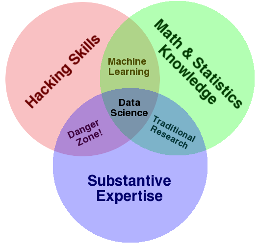
Next: What is political science?

The science of politics, of course! Politics focuses on studying governance and the distribution of power in society, broadly conceived.
- How else might you define politics and political science? What do we study in political science?

1.1.2 Course Goals

Social Science Goals

We have several goals in social science. Here are four that data science can help us pursue:

Describe and measure
- Has the U.S. population increased?
Explain, evaluate, and recommend (study of causation)
- Does expanding Medicaid improve health outcomes?
Predict
- Who will win the next election?
Discover
- How do policies diffuse across states?

What are other examples of these goals?

Note: In this course, we are exploiting the benefits of quantitative data to help achieve goals of social science. However, quantitative data have their shortcomings, too. We will also discuss the limitations of various applications of social science data, and we encourage you to always think critically about how we are using data.

This course will provide you with a taste of each of these social science goals, and how the use of data can help achieve these goals. By the end of the course, you should be able to

Provide examples of how quantitative data may be used to help answer social science research questions.
Compare and contrast the goals of description, causation, prediction, and discovery in social science research.
Use the programming language R to import and explore social science data and conduct basic statistical analyses.
Interpret and describe visual displays of social science data, such as graphs and maps.
Develop your own analyses and visualizations to understand social science phenomena.

If you are someone that loves data, we hope you will find this course engaging. If you are someone who loathes or finds the idea of working with data and statistics alarming, we hope you keep an open mind. We will meet you where you are. This course will not assume knowledge of statistical software, and there will be plenty of opportunities to ask questions and seek help from classmates and the instructor throughout the semester.

The first section of course will walk people through how to use the statistical program– R– that we will employ this semester.

Will this course help me in the future?

Even if you do not plan on becoming a social scientist or a data scientist, an introduction to these skills may prove helpful throughout your academic and professional careers.

To become an informed consumer of news articles and research involving quantitative analyses.
To practice analytical thinking to make informed arguments and decisions.
To expand your toolkit for getting a job that may involve consuming or performing some data analysis, even if that is not the traditional role.
- Example: Journalism- How 5 Data Dynamos Do Their Jobs

1.2 Setup in R

Goal

By the end of the first week of the course, you will want to have R and RStudio installed on your computer (both free), feel comfortable using R as a calculator, and making documents using the R Markdown file type within RStudio.

R is an application that processes the R programming language. RStudio is also an application, which serves as a user interface that makes working in R easier. We will primarily open and use RStudio to work with R.

In other classes, you may come across Stata, SPSS, Excel, or SAS, which are programs that also conduct data analysis. R has the advantage of being free and open-source. Even after you leave the university setting, you will be able to use R/RStudio for free. As an open-source program, it is very flexible, and a community of active R/RStudio users is constantly adding to and improving the program. You might also encounter the Python language at some point. R and Python have similarities, and learning R can also make learning Python easier down the road.

R and RStudio Installation

This content follows and reinforces section QSS 1.3 in our book. Additional resources are also linked below.

This video from Professor Christopher Bail explains why many social scientists use R and describes the R and RStudio installation process. This involves
1. Going to cran, select the link that matches your operating system, and then follow the installation instructions, and
2. Visiting RStudio and follow the download and installation instructions. R is the statistical software and programming language used for analysis. RStudio provides a convenient user interface for running R code.

1.3 Open R Script in RStudio

This next section provides a few notes on using R and RStudio now that you have installed it. In this section, we cover the following materials:

Using R as a calculator and assigning objects using <-
Setting your working directory and the setwd() function.
Creating and saving an R script (.R file)
Creating, saving, and compiling an R Markdown document (.Rmd) into an html document (.html)

This section highlights important concepts from QSS chapter 1.

RStudio is an open-source and free program that greatly facilitates the use of R, especially for users new to programming. Once you have downloaded and installed R and RStudio, to work in R, all you need to do now is open RStudio (it will open R). It should look like this, though your version numbers will be different:

Note: The first time you open RStudio, you likely only have the three windows above. We will want to create a fourth window by opening an R script to create the fourth window.

To do this, in RStudio, click on File -> New -> R script in your computer’s toolbar. This will open a blank document for text editing in the upper left of the RStudio window. We will return to this window in a moment.
- You can alternatively click on the green + sign indicator in the top-left corner of the RStudio window, which should give you the option to create a new R script document.

Now you should have something that looks like this, similar to Figure 1.1. in QSS:

The upper-left window has our .R script document that will contain code.
The lower-left window is the console. This will show the output of the code we run. We will also be able to type directly in the console.
The upper-right window shows the environment (and other tabs, such as the history of commands). When we load and store data in RStudio, we will see a summary of that in the environment.
The lower-right window will enable us to view plots and search help files, among other things.

1.3.1 Using R as a Calculator

The bottom left window in your RStudio is the Console. You can type in this window to use R as a calculator or to try out commands. It will show the raw output of any commands you type. For example, we can try to use R as a calculator. Type the following in the Console (the bottom left window) and hit “enter” or “return” on your keyboard:

5 + 3

[1] 8

5 - 3

[1] 2

5^2

[1] 25

5 * 3

[1] 15

5/3

[1] 1.666667

(5 + 3) * 2

[1] 16

Again, in the other RStudio windows, the upper right will show a history of commands that you have sent from the text editor to the R console, along with other items. The lower right will show graphs, help documents and other features. These will be useful later in the course.

1.3.2 Working in an R Script

Earlier, I asked you to open an R script in the upper left window by doing File, then New File, then R Script. Let’s go back to working in that window.

Set your working directory setwd()

Many times you work in RStudio, the first thing you will do is set your working directory. This is a designated folder in your computer where you will save your R scripts and datasets.

There are many ways to do this.

An easy way is to go to Session -> Set Working Directory -> Choose Directory. I suggest choosing a folder in your computer that you can easily find and that you will routinely use for this class. Go ahead and create/select it.
Note: when you selected your directory, code came out in the bottom left Console window. This is the setwd() command which can also be used directly to set your working directory in the future.
If you aren’t sure where your directory has been set, you can also type getwd() in your Console. Try it now

## Example of where my directory was
getwd()

[1] "/Users/ktmccabe/Dropbox/GitHub2/dsps23"

If I want to change the working directory, I can go to the top toolbar of my computer and use Session -> Set Working Directory -> Choose Directory or just type my file pathway using the setwd() below:

## Example of setting the working directory using setwd().
## Your computer will have your own file path.
setwd("/Users/ktmccabe/Dropbox/Rutgers Teaching/")

1.3.3 Saving the R Script

Let’s now save our R script to our working directory and give it an informative name. To do so, go to File, then Save As, make sure you are in the same folder on your computer as the folder you chose for your working directory.

Give the file an informative name, such as: “McCabeWeek1.R”. Note: all of your R scripts will have the .R extension.

1.3.4 Annotating your R script

Now that we have saved our R script, let’s work inside of it. Remember, we are in the top-left RStudio window now.

Just like the beginning of a paper, you will want to title your R script. In R, any line that you start with a # will not be treated as a programming command. You can use this to your advantage to write titles/comments– annotations that explain what your code is doing. Below is a screenshot example of a template R script.
You can specify your working directory at the top, too. Add your own filepath inside setwd()

Then you can start answering problems in the rest of the script.
Think of the R script as where you write the final draft of your paper. In the Console (the bottom-left window), you can mess around and try different things, like you might when you are taking notes or outlining an essay. Then, write the final programming steps that lead you to your answer in the R script. For example, if I wanted to add 5 + 3, I might try different ways of typing it in the Console, and then when I found out 5 + 3 is the right approach, I would type that into my script.

1.3.5 Running Commands in your R script

The last thing we will note in this section is how to execute commands in your R script.

To run / execute a command in your R script (the upper left window), you can

Highlight the code you want to run, and then hold down “command + return” on a Mac or “control + enter” on Windows
Place your cursor at the end of the line of code (far right), and hit “command + return” on a Mac or “control + return” on Windows, or
Do 1 or 2, but instead of using the keyboard to execute the commands, click “Run” in the top right corner of the upper-left window.

Try it: Type 5 + 3 in the R script. Then, try to execute 5 + 3. It should look something like this:

After you executed the code, you should see it pop out in your Console:

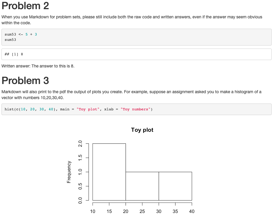
5 + 3

[1] 8

Note: The symbol # also allows for annotation behind commands or on a separate line. Everything that follows # will be ignored by R. You can annotate your own code so that you and others can understand what each part of the code is designed to do.

## Example
sum53 <- 5 + 3 # example of assigning an addition calculation

1.3.6 Objects

Sometimes we will want to store our calculations as “objects” in R. We use <- to assign objects by placing it to the left of what we want to store. For example, let’s store the calculation 5 + 3 as an object named sum53:

sum53 <- 5 + 3

After we execute this code, sum53 now stores the calculation. This means, that if we execute a line of code that just has sum53, it will output 8. Try it:

sum53

[1] 8

Now we no longer have to type 5 + 3, we can just type sum53. For example, let’s say we wanted to subtract 2 from this calculation. We could do:

sum53 - 2

[1] 6

Let’s say we wanted to divide two stored calculations:

ten <- 5 + 5
two <- 1 + 1
ten / two

[1] 5

The information stored does not have to be numeric. For example, it can be a word, or what we would call a character string, in which case you need to use quotation marks.

mccabe <- "professor for this course"
mccabe

[1] "professor for this course"

Note: Object names cannot begin with numbers and no spacing is allowed. Avoid using special characters such as % and $, which have specific meanings in R. Finally, use concise and intuitive object names.

GOOD CODE: practice.calc <- 5 + 3
BAD CODE: meaningless.and.unnecessarily.long.name <- 5 + 3

While these are simple examples, we will use objects all the time for more complicated things to store (e.g., like full datasets!) throughout the course.

We can also store an array or “vector” of information using c()

somenumbers <- c(3, 6, 8, 9)
somenumbers

[1] 3 6 8 9

Importance of Clean Code

Ideally, when you are done with your R script, you should be able to highlight the entire script and execute it without generating any error messages. This means your code is clean. Code with typos in it may generate a red error message in the Console upon execution. This can happen when there are typos or commands are misused.

For example, R is case sensitive. Let’s say we assigned our object like before:

sum53 <- 5 + 3

However, when we went to execute sum53, we accidentally typed Sum53:

Sum53

Error in eval(expr, envir, enclos): object 'Sum53' not found

Only certain types of objects can be used in mathematical calculations. Let’s say we tried to divide mccabe by 2:

mccabe / 2

Error in mccabe/2: non-numeric argument to binary operator

A big part of learning to use R will be learning how to troubleshoot and detect typos in your code that generate error messages.

1.4 R Markdown

An R Markdown document, which you can also create in RStudio, allows you to weave together regular text, R code, and the output of R code in the same document. This can be very convenient when conducting data analysis because it allows you more space to explain what you are doing in each step. We will use it as an effective platform for writing up problem sets.

R Markdown documents can be “compiled” into html, pdf, or docx documents by clicking the Knit button on top of the upper-left window. Below is an example of what a compiled html file looks like.

Note that the image has both written text and a gray chunk, within which there is some R code, as well as the output of the R code (e.g., the number 8 and the image of the histogram plot.

We say this is a “compiled” RMarkdown document because it differs from the raw version of the file, which is a .Rmd file format. Below is an example of what the raw .Rmd version looks like, compared to the compiled html version.

1.4.1 Getting started with RMarkdown

Just like with a regular R script, to work in R Markdown, you will open up RStudio.

For additional support beyond the notes below, you can also follow the materials provided by RStudio for getting started with R Markdown https://rmarkdown.rstudio.com/lesson-1.html.

The first time you will be working in R Markdown, you will want to install two packages: rmarkdown and knitr. You can do this in the Console window in RStudio (remember the lower-left window!).

Type the following into the Console window and hit enter/return.

install.packages("rmarkdown")
install.packages("knitr")

Once you have those installed, now, each time you want to create an R Markdown document, you will open up a .Rmd R Markdown file and get to work.

Go to File -> New File -> R Markdown in RStudio
- Alternatively, you can click the green + symbol at the top left of your RStudio window
This should open up a window with several options, similar to the image below
- Create an informative title and change the author name to match your own
- For now, we will keep the file type as html. In the future, you can create pdf or .doc documents. However, these require additional programs installed on your computer, which we will not cover in the course.

After you hit “OK” a new .Rmd script file will open in your top-left window with some template language and code chunks, similar to the image below. Alternatively, you can start from scratch by clicking “Create Empty Document” or open a template .Rmd file of your own saved on your computer.

Save as .Rmd file. Save the file by going to “File -> Save as” in RStudio

Give the file an informative name like your LastnamePractice1.Rmd

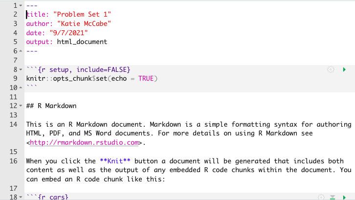
Key Components. Now you are ready to work within the Rmd script file. We will point to four basic components of this file, and you can build your knowledge of RMarkdown from there.
1. The top part bracketed by --- on top and bottom is the YAML component. This tells RStudio the pertinent information about how to “compile” the Rmd file.
  - Most of the time you can leave this alone, but you can always edit the title, author, or date as you wish.
2. The next component are the global options for the document. It is conveniently labeled “setup.” By default what this is saying is that the compiled version will “echo” (i.e., display all code chunks and output) unless you specifically specify otherwise. For example, note that it says include = FALSE for the setup chunk. That setting means that this code chunk will “run” but it will not appear in the nicely compiled .html file.
  - Most of the time you will not need to edit those settings.
3. The third component I want to bring attention to is the body text. The # symbol in RMarkdown is used to indicate that you have a new section of the document. For example, in the compiled images at the beginning, this resulted in the text being larger and bolded when it said “Problem 2.” In addition to just using a single #, using ## or ### can indicate subsections or subsubsections. Other than that symbol, you can generally write text just as you would in any word processing program, with some exceptions, such as how to make text bold or italicized.
4. The final component I want to call attention to are the other main body code chunks. These are specific parts of the document where you want to create a mini R script. To create these, you can simply click the + C symbol toward the top of the top left window of RStudio and indicate you want an R chunk.
Writing R Code. Within a code chunk, you can type R code just like you would in any R script, as explained in the previous section. However, in RMarkdown, you also have the option of running an entire code chunk at once by hitting the green triangle at the top-right of a given code chunk.

Knitting the document. Once you have added a code chunk and/or some text, you are ready to compile or “Knit” the document. This is what generates the .html document.
- To do so, click on the Knit button toward the top of the top-left window of Rstudio. After a few moments, this should open up a preview window displaying the compiled html file.
- It will also save an actual .html file in your working directory (the same location on your computer where you have saved the .Rmd file)
- Try to locate this compiled .html file on your computer and open it. For most computers, .html files will open in your default web browser, such as Google Chrome or Safari.
- This step is a common place where errors are detected and generated. Sometimes the compiling process fails due to errors in the R code in your code chunks or an error in the Markdown syntax. If your document fails to knit, the next step is to try to troubleshoot the error messages the compiling process generates. The best way to reduce and more easily detect errors is to “knit as you go.” Try to knit your document after each chunk of code you create.

1.5 Assignment 1

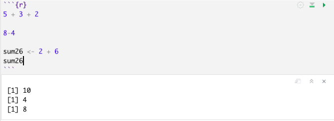
Below is an exercise that will demonstrate you are able to use R as a calculator, create R scripts, and create and compile R Markdown files.

We will start walking through this assignment together during class, but you are welcome to try to do this ahead of time on your own.

You will submit three documents on Canvas:

An R script (.R) file with your code. Follow the best practices by titling your script and using # comments to explain your steps. This code should be clean. I should be able to run your code to verify that the code produces the answers you write down.
An .Rmd document and a compiled RMarkdown .html document that you get after “knitting” the .Rmd file. This should also have a title including your name and use text or # comments to explain your steps.

You can create these documents from scratch using the guidance in the previous sections, or you can download and open the .R and .Rmd templates, provided on Canvas, in RStudio to get started. This video provides a brief overview of opening an R script and R Markdown file in RStudio. The notes provide additional details.

Assignment Exercises

Create a .R script saved as “LastnameSetup1.R” (use your last name). Within this file, make sure to title it and provide your name.
1. Set your working directory, and include the file pathway (within setwd()) at the top of your .R script
2. Do the calculation 8 + 4 - 5 in your R script. Store it as an object with an informative name. Report the answer as a comment # below the code.
3. Do the calculation 6 x 3 in your R script. Store it as an object with an informative name. Report the answer as a comment # below the code.
4. Add these two calculations together. Note: do this by adding together the objects you created, not the underlying raw calculations. Report the answer as a # below the code.
In this problem, we will just re-format what we did in the first problem in an R Markdown format. Create a .Rmd R Markdown file saved as “LastnameSetup1.Rmd.” Within this file, make sure to title it and provide your name.
1. Create a Markdown heading # Problem 2.1. Underneath this, create an R code chunk in which you do the calculation 8 + 4 - 5. Store it as an object with an informative name. Report the answer in plain language below the code chunk.
2. Create a Markdown heading # Problem 2.2. Underneath this, create an R code chunk in which you do the calculation 6 x 3 in your R script. Store it as an object with an informative name. Report the answer in plain language below the code chunk.
3. Create a Markdown heading # Problem 2.3. Underneath this, create an R code chunk in which you add the previous two calculations together. Note: do this by adding together the objects you created, not the underlying raw calculations. Report the answer in plain language below the code chunk.
4. Create a Markdown heading # Problem 2.4. Write down how you will complete your R assignments this semester. For example, if you have a personal laptop with R and RStudio on it, you will simply write “I will use my personal laptop.” If you don’t have a personal computer or laptop, please indicate where on campus or off-campus you will have regular access to a computer with R/RStudio to do your work. It is essential that you have regular access to a computer so that you will not fall behind in this course.
Create a compiled .html file by “knitting” the .Rmd file into a .html document. Save the file as “LastnameSetup1.html.”

All done! Submit the three documents on Canvas.